How Transformers Attend — Part I
At a glance
🚀 Start here: Theorem K.1: Nulo uniforme y calibración de la pendiente.
Main results:
- Proposition 5.1: La suma de cosenos no implica el candidato Padé
- Theorem 6.1: MaxEnt selecciona una familia de potencias bajo un momento fijado
- Theorem 6.2: Existencia y unicidad del exponente MaxEnt en soporte finito
- Theorem 7.2: Entropía de la familia finita y sus regímenes asintóticos
- Theorem 11.1: Cuantil continuo de masa y cuantil discreto de tokens
- Theorem K.1: Nulo uniforme y calibración de la pendiente
- Theorem K.2: Sesgo de exposición afín
- Theorem K.3: Curvatura de mezclas de potencias
- Theorem K.4: Orden de cuantiles en soporte finito
- Theorem K.5: Identidades de la familia exponencial finita
- Theorem K.6: Cotas de truncación para una fila congelada
- Theorem K.7: Estabilidad del softmax ante cambios de puntaje
- Theorem K.8: Integral coseno y residuo RoPE explícito
🗺️ Map of the results (click a box to go to it)
Dependencies in the written proof: an arrow A → B means that this proof of B uses A. Every result rests on its written proof; the tags record what was checked besides, and each statement's “Evidence & scope” block says how far. The colour of a box is its strongest tag, in the order above; the tags in the box give the rest. Boxes with a thick border are the main results; click a box to read the statement.
📐 Setting (from the paper, Section 1.4)
Within the normalized family, larger \(\gamma \) shifts mass toward shorter distances. For a general model, a fitted \(\widehat\gamma \) describes only the profile and interval on which it was estimated. A configuration value \(\gamma _P\) is a separate candidate. The exploratory five-axis regression in Section 5.5, with reported \(R^2=0.44\), describes the initial panel; its coefficients do not identify separate causal contributions.
Corrected English edition: formal results integrated, 19 November 2026
Known algebraic, numerical, implementation-description and cross-reference errors identified in the audit are corrected in this edition. Unsupported physical identifications and performance guarantees have been withdrawn. Superseded prose, tables and controller code remain in the separate source archive; they are not reproduced as an alternative set of conclusions here. Appendix J records the resolutions. A new reference implementation repairs prefix causality, head-projection placement, rotary pairing and the context-input interface, with synthetic checks described in Section 19.3. Those checks do not replace the archived model results or establish trained-model efficacy. Unavailable historical observations are identified as missing evidence; no values have been invented to fill them. Appendix K adds eight groups of mathematical results with their verified Isabelle/HOL proofs and explicit hypotheses.
Abstract.
A measured profile and a conditional mathematical family. This corrected edition studies attention-distance profiles, the finite power-law family \(p_\gamma (d)=d^{-\gamma }/Z_N(\gamma )\), and the applications originally proposed within the Thermodynamic Attention Framework (TAF). It preserves the original subject matter and detailed evidence while correcting the inference from rotary geometry to a universal trained exponent. RoPE gives an exact sine–cosine score decomposition. It does not, without further assumptions on learned queries and keys, impose a log-distance expectation or the maximum-entropy principle. The proposed configuration formula \(\gamma _P=(2\theta -T\sqrt2)/(2\theta +T\sqrt2)\) remains an algebraic candidate; its stationary-phase derivation is withdrawn because an essential logarithmic ratio equals \(-1\) rather than the proposed variable exponent.
Instrument dependence. The initial E4 procedure changes sequence length with distance. Its actual extractor returns \(\widehat\gamma =0.782582\) with \(R^2=0.988452\) on uniform causal attention over the seven-point 30–2000 grid. Thus a good power-law fit does not identify learned decay or validate the Padé candidate. In contrast, the audited October QL estimator uses fixed query positions and has zero uniform-null slope on its fitted range. These are synthetic instrument checks, not new model measurements. The initial and October protocols remain distinct.
Coordinate and field controls. The available B3 masks remove unequal sets of adjacent coordinates, not complementary rotary planes. The GPU amplification code also modifies V. The separate field estimator uses \(d+60\) tokens and gives a uniform-null slope \(0.755252\), close to the initial checkpoint’s \(0.757234\). Archived effects therefore do not establish a learned geometric optimum, semantic reservoir or functional interpretation of the spectral ratio.
Empirical record and its update. The original model panels, corpus contrasts, ablations and negative results are retained with their historical status. The selected-case accuracy statistic is withdrawn because its row membership and selection record could not be reconstructed (Section 5.4). A saved-data replay reconstructs October fits and sequence-bootstrap intervals for 25 of 42 historical model identifiers: 15 at context 2048 and ten at 1024; 17 have no recovered observation. The historical text exponent falls inside the corresponding interval in one of 25 cases. Spearman correlation is \(0.269\) between historical and QL exponents, and \(-0.445\) between 19 stored Padé values and QL exponents. Changes in corpus, precision and protocol prevent assigning all discrepancies to one cause. Only four successful job records contain an immutable weight revision. Replaying arrays is not an end-to-end replication of inference.
Mathematics retained with explicit hypotheses. On a finite discrete support, maximum entropy at an interior prescribed log-distance moment has a unique power-law optimizer with a real exponent. Positivity requires the moment to lie below its uniform-distribution value. Exact finite sums determine the normalizer, entropy, Fisher information and formal heat capacity. The continuous variance \((\log N)^2/12\) at \(\gamma =1\) is not the discrete value: at \(N=2000\) they are \(4.81448\) and \(5.48412\), respectively. The Fisher metric obeys \(C_V=\gamma ^2I\); the intrinsic length integrates \(\sqrt I\), and the two quantities need not peak together. The finite continuous mass quantile is well defined on both sides of one, with value \(N^f\) at one; the token-distance quantile instead uses partial sums.
Applications and limits. The compression experiments, context-extension tests, per-head profiles, alignment comparisons, circuit hypotheses and architectural descriptions remain available in their original sections. A frozen-row output error can be bounded from removed mass and value diameter, but that bound does not certify autoregressive task accuracy. Inverse Padé returns its input context exactly and therefore cannot independently validate a retrieval horizon. Divergence from a normalized positional null does not by itself identify a circuit. Geometric band counts require the actual rotary subspace and pairing convention; completion of a cycle does not establish loss of information. The remaining analogy and score definitions have explicit domains and no claimed physical identification or calibrated predictive interpretation. The corrected intervention reference is distinguished from the defective historical implementations and their archived aggregate scores.
The November campaign adds 8,064 saved interventions on 32 shared prompts for three models. The reported gradient-prediction gains concern error prediction, not improved model capability. Appendix K integrates eight formally verified groups on instrument nulls, affine exposure, mixtures, quantiles, finite-family sensitivity, truncation, softmax and the conditional RoPE approximation. Their proofs establish the stated mathematical implications, not the empirical pipeline or bibliographic novelty. The companion Blueprint maps the statements, proofs, figures and interactive calculations of this edition. TAF Agent and the field guide provide application and measurement routes; their outputs are not independent validation of the empirical claims.
[colback=ModernTint,colframe=ModernInk, title=Reader’s Guide: Three Tracks Through This Paper]
The manuscript distinguishes measured attention profiles, conditional results for a finite power-law family, and intervention hypotheses. Geometry alone does not connect these three levels into a validated causal chain.
(T) Mathematical track. Read Sections 4–7 for the rotary identity, the candidate exponent, maximum entropy under a prescribed moment, and finite thermodynamic quantities. Section 7.4 separates the finite entropy bound from its asymptotic regimes. The physical identifications in Section 20 are retained historical hypotheses, subject to their local corrections, rather than consequences of these theorems.
(E) Empirical and engineering track. Start with Sections 2, 8 and 9. Then read Sections 11 and 12 for mass quantiles, recorded compression trials and inverse-candidate algebra. These calculations require protocol-specific measurements and task evaluation before use as intervention rules. Appendix E gives the current checklist. Section 21 preserves the historical application; its interface is not independent validation of the manuscript.
(F) Full research record. Read sequentially for the observations, proposed mechanisms, negative results and corrections. Sections 18 and 18.1, and Appendix F, record failures and unresolved tests. Appendix J records the corrections and the location of the separate historical archive. The obsolete recipes are absent from this corrected edition.
1 Introduction
1.1 An Empirical Regularity
Measurement qualification.
The initial empirical pattern must be read with the instrument control in Section 9.1. Under its variable-length sampling rule, uniform causal attention already gives a fitted exponent near \(0.78\). The pattern alone does not establish learned decay, a rotary mechanism or a universal exponent. Fixed-query QL uses a different null and protocol.
Attention-distance profiles summarize how a model distributes attention over token separations under a specified corpus, context and estimator. The family
provides a compact description of some such profiles. Its adequacy is an empirical question: an arbitrary softmax of learned dot products need not have this form. A high log-log \(R^2\) on a selected distance interval does not establish the same law at attention sinks, at every head, or outside that interval.
The initial model panel spans Pythia-14M to BLOOM-7b1 and includes RoPE, ALiBi and learned positional encodings. In the replayed 21-row panel, P03, P05 and P07 have \(R^2{\lt}0.95\); the other 18 exceed it. This panel motivated the configuration-only candidate studied in Section 5, whose accuracy must be assessed on an explicitly identified set of observations. Corpus, precision, architecture, training and measurement choices must be considered when comparing fitted exponents.
The saved October measurements supply a second, explicitly defined comparison (Section 8). Fits and sequence-bootstrap intervals can be recomputed for 25 of 42 model identifiers: 15 at context 2048 and ten at 1024. Seventeen identifiers lack recovered observations. One of the 25 initial text exponents lies in the corresponding interval. The Spearman correlations are \(0.269\) between initial and recomputed exponents and \(-0.445\) between 19 stored Padé values and recomputed exponents. These comparisons demonstrate sensitivity to the measurement protocol; because several conditions changed together, they do not identify a single causal source of the differences. Only four successful job records identify an immutable weight revision. Recomputing saved arrays therefore verifies the reported calculations, not the entire inference pipeline.
One-line summary.
We measure distance profiles, analyze a conditional finite power-law family, and test specific interventions. The geometric description, the mathematical family and the empirical response are connected by explicit hypotheses and comparisons, rather than by an assumed universal exponent.
1.2 Four Questions
Why consider a power law? For a prescribed feasible log-distance moment on finite support, maximum entropy selects a power law. Whether measured attention meets this optimization premise requires evidence.
What determines \(\gamma \)? A measured exponent depends on the model and protocol. We compare it with a configuration-based Padé candidate; RoPE alone does not derive their equality.
What is special about \(\gamma =1\)? It separates the summability regimes of the infinite-support family. At any finite context the normalizer, entropy and variance remain finite and smooth. Continuous and discrete quantiles must be distinguished.
What can we do with \(\gamma \)? Profiles and conditional bounds can guide compression, context-extension and anomaly experiments. Task-level benefits must be measured under the intervention actually performed.
1.3 The Theoretical Chain
The argument starts with three separate objects. First, RoPE supplies a set of rotation frequencies and an exact sine–cosine decomposition of attention scores. Second, a specified log-distance moment defines a constrained inference problem. Third, measurements determine whether a particular trained model is described adequately by the resulting family.
For integer \(N{\gt}1\) and an interior feasible moment \(0{\lt}\lambda {\lt}\log N\), maximizing Shannon entropy over distributions on \(\{ 1,\ldots ,N\} \) with \(\mathbb E_p[\log d]=\lambda \) selects a unique power law. Its exponent is a real Lagrange multiplier, positive only below the uniform log moment \(\log (N!)/N\). The Gibbs-inequality argument and the precise hypotheses are given in Section 6. Other distributions can share the prescribed moment without maximizing entropy. The frequency geometry does not impose either the moment or the optimization principle on trained queries and keys.
This distinction also limits the proposed geometric prediction. A rational function of configuration variables can be evaluated without inference, but that computational convenience does not make it a derived trained exponent. Section 5 analyzes the candidate, the unsuccessful derivation and the empirical comparisons separately. All downstream uses retain this boundary.
1.4 The Central Object
Within the normalized family, larger \(\gamma \) shifts mass toward shorter distances. For a general model, a fitted \(\widehat\gamma \) describes only the profile and interval on which it was estimated. A configuration value \(\gamma _P\) is a separate candidate. The exploratory five-axis regression in Section 5.5, with reported \(R^2=0.44\), describes the initial panel; its coefficients do not identify separate causal contributions.
The geometric quantity is the number of rotary planes that have completed a cycle. For \(m=d_{\rm rot}/2\), \(d{\gt}0\) and \(\theta {\gt}1\), define
Here \(n_\mathrm {active}\) counts planes without a complete cycle, not information-bearing dimensions. The actual rotary subspace and coordinate pairing must be used. The continuous logarithmic count is an approximation to this integer count; it does not supply a trained attention exponent or an information-loss theorem.
1.5 The Many Faces of \(\gamma \)
The notation must distinguish quantities whose equality is not established.
|
Quantity |
Meaning and scope |
|
\(\widehat\gamma \) |
Estimated profile exponent, with protocol and uncertainty. |
|
\(\gamma \) |
Parameter of the finite probability family; identities are conditional on this model. |
|
\(\gamma _P\) |
Rational candidate computed from configuration, requiring empirical comparison. |
|
\(1/\gamma \) |
Formal inverse-temperature coordinate when \(\gamma \ne 0\), not the output sampling temperature. |
Architecture fingerprints are statistics formed from these quantities. Their diagnostic usefulness depends on the reference panel and validation protocol.
1.6 What This Paper Contributes
The paper develops the following connected analyses. Mathematical statements, derived calculations, model measurements and proposals carry different evidence.
Configuration candidate and its limits (Section 5). Building on measured attention-distance structure criticalattn2025,barbero2024roundandround, we analyze \(\gamma _P=(2\theta -T\sqrt2)/(2\theta +T\sqrt2)\), including its domain, inverse, comparison panel and failed stationary-phase argument. The initial comparison identifies all 13 computable residuals; the October comparison uses its own protocol.
Conditional maximum entropy (Section 6). We specify the support, reference measure and feasible moment, derive the optimizing family, and distinguish its entropy \(S=\log Z+\gamma \mathbb E[\log d]\) from measured attention entropy.
Finite and asymptotic regimes (Section 7). Exact sums separate finite-context calculations from infinite-support limits and continuous approximations. Comparisons of compressibility between models remain observations, not universal ratios.
KV compression (Section 11). We derive continuous and discrete mass windows and a frozen-row output bound. The experiments retain the windows actually tested: EXP-B2 used 445 tokens for Pythia-1B and 1482 for Pythia-2.8B. The soft-decay comparison favors different policies on its three models; its percentages depend on the stated denominator. The unsuccessful cases remain part of the evidence, and none establishes general accuracy guarantees.
Context extension (Section 12). EXP-B1v5 compares four Pythia models at \(\alpha \in \{ 1,4,8,16\} \) and nominal lengths 512–4096. At 4096, \(\alpha =4\) scores \(86,100,100,100\% \) in restricted key ranking. It does not dominate every setting and incurs small recorded short-context losses on Pythia-70M. The small-model panel duplicates v4; nominal chance is not a measured control. Neither an optimum nor fine-tuning performance follows from these aggregates.
Entropy and band interventions (Sections 7.4 and 13). The finite entropy bound is mathematical; the replayed finite-family calculations are tabulated in Section 8. EXP-B3 reported perplexity increases of 350 and 9.3 on Pythia-1B for two sets of ablated weight rows. The ratio from the unrounded records is \(37.45\) (approximately \(37\times \)). This contrast motivates a band hypothesis, whose causal interpretation requires correct pairing and partial-RoPE controls.
Attention anomalies (Section 14). Divergence from a normalized positional reference identifies departures from that reference. Circuit identification additionally requires functional interventions.
Measurement workflow and model panels (Sections 9 and 17). The model tables, measurement software and protocol records support reproducible comparisons. Available and missing observations are reported explicitly.
Control proposals (Sections 3 and 19). We separate RoPE changes, score temperature, training and output sampling. The proposed bands below \(0.65\), from \(0.65\) to \(0.85\), and above \(0.85\) are exploratory design choices. A thermostat requires prospective task evaluation.
Information geometry and physical analogies (Sections 7.3 and 20). The finite-family identity \(C_V=\gamma ^2 I\) and rational-map derivatives have explicit mathematical domains. Fractional-operator, conformal and renormalization interpretations are assessed against the additional structures they would require.
Intervention evidence (Section 19.2). The adaptive historical hooks fail prefix causality; their reported scores and the former Fisher recovery comparison cannot validate causal performance. The November campaign supplies 8,064 interventions on 32 shared prompts for three models, including controls and paired uncertainty. Predictor-error reductions are not improvements in model capability.
Failure analysis (Section 20.9 and Appendix F). The proposed geometric hallucination scores lack factual-error calibration. Their domain failures and the unsuccessful controller and physical hypotheses delimit what the framework can support.
Reader’s map.
Sections 5–7 separate candidate geometry from conditional mathematics; Section 8 presents the measurement panels and replay. Sections 11–12 and 19 contain intervention applications. The diagnostics, architecture comparisons and software descriptions retain their detailed methods and examples. The formula catalogue and compendium organize the results with their domains; the separate change and evidence document records version history and the exact scope of formal certificates.
1.7 Relation to Prior Work
Attention profiles and rotary geometry.
Work on attention-distance structure and rotary representations criticalattn2025,barbero2024roundandround,attngravity2026,su2024roformer provides context for the profile measurements examined here. This manuscript does not establish a first-principles exponent for learned attention. Its conditional maximum-entropy result and configuration candidate have different premises and must be assessed separately from the empirical fits.
Context extension.
The context-extension literature studies rotary schedules and extrapolation yang2024understanding,ropebounds2024,ropedimension2025,ropemodulation2026,peng2023yarn,liu2023scaling. Hybrid positional schemes and rotary-dimension analyses provide further comparisons ropenopebackagain2025,shang2025rcdim. Inverting our candidate does not derive the optimal parameters of these methods or identify which layers can discard rotary information. Section 12 gives the precise inverse and separates it from the recorded retrieval experiments.
KV-cache compression.
SnapKV, H2O, StreamingLLM and PyramidKV use different selection or allocation mechanisms snapkv2024,zhang2023h2o,xiao2023streamingllm,cai2024pyramidkv. BLASST and reasoning-focused evaluations offer additional empirical comparisons blasst2025,holdontothat2025. Related compression and layer-skipping work includes mixcompressrefine2025,shortgpt2024,csordas2025layerskipping,elitekv2025. These methods do not all implement a distance-window quantile. Our conditional mass budget therefore does not explain a universal operating point or replace their calibration. In particular, the previously asserted BLASST coefficient and PyramidKV retention match were incorrect; the corrected algebra and numerical comparison are in Section 11.4.
Positional diagnostics and circuits.
Studies of positional and symbolic attention deconstructpositional2025,decouplepsymbolic2025,barbero2024roundandround motivate hypotheses about rotary bands. Here the observed band-ablation asymmetry is retained, with instrument limitations, rather than presented as a proof of a semantic reservoir. Likewise, a corpus contrast or KL departure from a positional null is a descriptive diagnostic. Transformer-circuit and induction-head work elhage2021mathematical,olsson2022induction, and activation-patching methods meng2022locating,heimersheim2024how, motivate additional causal tests; a sign reversal alone does not identify their circuits.
Entropy and physical analogies.
Attention entropy, frequency-domain diagnostics and attention scaling are studied under different definitions and limits emnlp2025entropy,dope2025,criticalattn2025. Statistical-mechanical approaches to weights, training, generation or attention paths provide related but distinct objects soc2026,phasetransform2025,phasetransformsmall2025,cui2024phasetransition,nakaishi2024critical,attndissect2024,kim2026thermodynamic. Our \(Z_N\) is a finite sum; its infinite-support limit is \(\zeta (\gamma )\) only for \(\gamma {\gt}1\). The family inverse-temperature coordinate is not the model’s output sampling temperature.
The finite Shannon bound \(S_N\le \log N\) does not identify an entanglement entropy or establish a geometric area law for trained attention. Ryu–Takayanagi theory and work on learning its inverse mapping ryu2006holographic,jhep2026rttransformer do not validate that inference. No claim of being the first derivation from positional geometry is supported by the corrected argument. Historical comparisons and their original wording remain in the separate predecessor archive indexed by Appendix J.
1.8 How to Read This Paper
The dependency diagram in Figure 3 distinguishes conditional mathematics from empirical tests. The entry points in Table 1 complement the reader guide at the start of the document.
|
Reader |
Start with |
Check alongside |
|
ML researcher |
Profiles and candidate comparisons, Sections 5, 8 |
Protocol limitations and negative results. |
|
Mathematical reader |
Finite-family results, Sections 6–7 |
Support, reference measure and fixed-exponent limits. |
|
Compression engineer |
Quantiles and interventions, Sections 11–12 |
Actual task and resource evaluation. |
|
Reader auditing history |
Appendix J and the source archive |
Correction register and exact predecessor source. |
Appendix E gives a measurement and evaluation checklist; Appendix G states the current status of F1–F20. They do not promise model-independent runtimes, production safety or novelty. The physical analogies and historical software descriptions elsewhere require their local qualifications, even where the original terminology is retained.
2 Summary of Results
The supported results have three distinct forms: identities within a specified probability family, computations reproduced from archived arrays, and empirical observations under recorded protocols. An identity evaluated at a fitted exponent is not an additional independent measurement of a model.
tableSupported results and the evidence that supports them.
|
Result |
What is established |
Evidence and scope |
|
Maximum entropy |
Unique power-law optimizer at an interior prescribed log moment. |
Theorems in Section 6; a conditional inference statement. |
|
Finite-family calculus |
Exact moments, entropy, Fisher information, heat capacity and discrete mass quantiles. |
Sections 7 and 11; specified support and parameter. |
|
Instrument controls |
Variable-length E4 has a nonzero uniform-null slope; fixed-query QL has zero slope. |
Section 9.1; analytic and synthetic checks. |
|
Corrected reference code |
Declared causal, rotary, loss and numerical contracts pass 145 checks. |
Section 19; CPU tensor and arithmetic tests. |
|
November interventions |
8,064 saved interventions, 32 shared prompts, three models, including 1,152 zero-strength controls. |
Section 19; prediction of intervention effects, not improved model performance. |
Four quantities and their scope
tableCurrent scope of the four quantities previously presented as deployment tools.
|
Quantity |
Definition |
Interpretation |
|
Padé candidate |
\(\gamma _P=(2\theta -T\sqrt2)/(2\theta +T\sqrt2)\) |
Algebraic candidate in \((-1,1)\) for positive inputs; not a universal measured exponent. |
|
Mass window |
\(D_{f,N}=\min \{ k:\sum _{d=1}^k d^{-\gamma }\ge fZ_N\} \) |
Exact discrete quantile. The continuous analogue is given in Section 11; neither is a task-accuracy guarantee. |
|
Inverse base |
\(\theta _{\rm inv}=T\sqrt2(1+g)/(2(1-g))\) |
Solves \(\gamma _P=g\) for \(-1{\lt}g{\lt}1\). Its ratio to a nominal base is not a demonstrated NTK optimum. |
|
Corpus contrast |
\(\Delta \widehat\gamma =\widehat\gamma _{\rm random}-\widehat\gamma _{\rm text}\) |
Protocol-dependent difference. Its sign alone does not identify architecture or an induction circuit. |
Evidence at a glance
The initial predictor comparison has 18 model/corpus entries, of which 13 have a recorded base. On those 13, the mean absolute exponent error is \(0.167766\), and the median absolute relative error is \(19.2144\% \). The selected-case accuracy claim is withdrawn for the provenance reasons in Section 5.4. The separate October replay has 25 observations among 42 historical identifiers, including 17 unavailable observations. Only four successful job records identify an immutable weight revision. The historical text estimate lies inside the October interval in one of 25 comparisons; the stored Padé candidate and the October QL exponent have Spearman correlation \(-0.445\) on 19 available pairs. Differences in protocol prevent attributing these discrepancies to one cause.
On finite support, maximum entropy selects a unique power-law distribution at an interior prescribed log-distance moment. Entropy, Fisher information and formal heat capacity are computed by finite sums. They remain finite at \(\gamma =1\); the infinite-support summability boundary is not a demonstrated transition in finite-network capability. At \(N=2000\) and \(\gamma =1\), the discrete variance is \(5.48412\), compared with \(4.81448\) for the continuous density.
The November campaign records 8,064 interventions on 32 shared prompts for three models, including 1,152 zero-strength controls. Its improvements concern prediction of intervention effects, not improved model performance. Historical KV, retrieval, alignment and band-ablation experiments remain in their original sections with their protocol limitations.
How to use the results
Measure a profile under a declared protocol, compare alternative fitted families, and propagate its uncertainty into derived quantities. Test any proposed cache or rotary intervention against task and resource baselines. The manuscript establishes neither a configuration-only safe compression ratio nor a general context-extension or architecture-classification rule. Measurement time depends on model size, hardware and protocol; a universal three-minute CPU estimate is not supported.
3 \(\gamma \) as a Candidate Control Coordinate
3.1 From an observable to an intervention hypothesis
A fitted exponent describes an attention-distance profile under a specified corpus, support and aggregation. It does not determine the entire computation of a trained network. Within the finite family, for a statistic \(u\) independent of \(\gamma \), differentiation gives
For increasing \(u(d)\), this derivative is nonpositive: increasing the positive family exponent shifts mass toward shorter distances. This statement does not identify a model intervention that realises a chosen change in \(\gamma \). The former task bands at \(0.65\) and \(0.85\) have no established universal decision status. Their original interpretation is preserved in the separate predecessor archive, not used as a deployment classification here.
3.2 Three levers with different mechanisms
Choosing a frequency schedule before training, changing rotary frequencies at inference, and modifying individual attention heads are different interventions. They require separate controls. Attention-score temperature is also distinct from output sampling temperature. A covariance identity for the chosen family cannot predict the full response of learned queries, keys and downstream states. The per-head profiles in Section 14.3 motivate measurement at finer resolution, while their missing layers limit whole-model conclusions.
For the candidate alone,
Thus increasing \(\theta \) increases the candidate exponent at fixed \(T\). This corrects the direction of the earlier proposed controller; it does not prove that a trained model follows this derivative.
3.3 Candidate curves and historical observations
🖼️ Figure 1
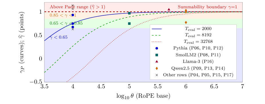
Candidate curves and retained historical fitted exponents. The curves evaluate \(\gamma _P\) at the three displayed contexts. The 13 points use the recorded bases and replayed exponents in Table 8; they are not measurements under a common context or corpus. The shaded bands preserve the old numerical intervals for orientation, without assigning task capability or a safe deployment regime. Points above one cannot be predictions of this candidate. Updated profile evidence is in Section 8.
The plot compares an algebraic family with historical fitted exponents. The curves and points do not constitute a controlled frequency-base sweep. Values above one can occur in a measured profile, although they cannot be outputs of this Padé candidate. The coloured intervals carry no established long-context, reasoning or training-stability guarantee.
3.4 A measurement and evaluation workflow
Define the task, evaluation context and baseline resource budget.
Record model, tokenizer and corpus revisions, attention backend, precision, query selection, support and estimator; estimate profile uncertainty.
Compute any family quantities on the stated support. Treat inverse Padé as a proposed experimental setting, not a task-optimal prescription.
Evaluate interventions on held-out sequences with paired baselines, recording both task quality and actual memory or latency changes.
The thermostat in Section 12.3 remains an unvalidated controller proposal. A measured response and a stability analysis are necessary before any runtime control claim.
4 Background and Notation
We distinguish the rotary map, a count of completed cycles, and distances derived from that count. None of these definitions alone determines the learned attention distribution.
4.1 Rotary Position Encoding
Let \(h=d_{\rm head}\) be the query/key head dimension and let \(d_{\rm rot}=2m\le h\), \(m\ge 1\), be the actual rotary dimension. Standard geometric RoPE su2024roformer rotates \(m\) two-dimensional planes. For \(\theta {\gt}1\) and zero-based plane index \(i\),
The frequencies range from \(1\) to \(\theta ^{-(m-1)/m}\). The slowest period is exactly \(2\pi \theta ^{(m-1)/m}\), approaching \(2\pi \theta \) only as \(m\to \infty \). Partial RoPE leaves \(h-2m\) coordinates unrotated; altered frequency schedules require their actual frequencies rather than this geometric formula.
For fixed content vectors \(q,k\) and rotations \(R\), orthogonality gives \((R(m_0)q)^\top R(n_0)k=q^\top R(n_0-m_0)k\). The explicit positional factor depends on the signed relative displacement. It need not be even in that displacement because the full score has a sine term. Content vectors can themselves depend on the surrounding context, so this identity does not imply that attention depends only on absolute distance or guarantee positional generalization.
Clock analogy. A plane records a phase modulo \(2\pi \) at every distance, including before its first full turn. Completing one turn is a threshold event in the unwrapped phase; it does not make the plane constant or erase all information in the joint vector of phases. Different clock readings can distinguish ideal positions, but usable discrimination also depends on weights, precision and noise.
4.2 Completed Cycles and the Uncycled-Plane Count
For real distance \(d{\gt}0\), call plane \(i\) cycled when \(d\omega _i\ge 2\pi \). The legacy symbols \(n_\mathrm {dead}\) and \(n_\mathrm {active}\) denote cycled and uncycled counts, respectively; they do not classify functional usefulness.
↳ Not used by another result of the paper.
Since \(\log \theta {\gt}0\), the threshold is equivalent to \(i\le x=m\log (d/2\pi )/\log \theta \). Among integers \(0,\ldots ,m-1\), the number satisfying this inequality is zero for \(x{\lt}0\), \(1+\lfloor x\rfloor \) for \(0\le x{\lt}m-1\), and \(m\) for \(x\ge m-1\). Clipping combines these cases and includes equality at the threshold. Subtracting from \(m\) gives the uncycled count.
En palabras.
El recuento separa los planos que han completado al menos una vuelta de los que aún no la han completado a una distancia dada. El umbral se calcula con las frecuencias rotatorias reales y se trunca entre cero y \(m\).
Alcance.
Completar una vuelta no significa perder información ni dejar de atender. El laboratorio de la Figura 2 comprueba el recuento exacto frente a la aproximación continua.
🧪 Lab: Figure 2 live: turn the rotary-cycle surface in 3D
Turn the exact uncycled-fraction surface over log distance and log RoPE base. The star marks your values; the flat curve below compares the integer count with its clipped continuous approximation. This counts geometric phase thresholds, not attention decay.
A convenient continuous approximation is
Its absolute error is at most one plane. For the fraction, the error is at most \(1/m\); relative error against a small or zero exact count has no uniform bound. The staircase and the clipped straight line are bookkeeping of phases, not a derivation of a power-law attention score. In particular, cycling does not imply that a coordinate contributes noise.
|
\(d\) |
\(n_\mathrm {dead}\) |
\(n_\mathrm {active}\) |
\(n_\mathrm {active}/m\) |
|
10 |
2 |
30 |
93.75% |
|
628 |
16 |
16 |
50% |
|
2,000 |
21 |
11 |
34.375% |
|
7,071 |
25 |
7 |
21.875% |
|
62,832 |
32 |
0 |
0% |
Colour: blue shade = the number’s size within its column.
🖼️ Figure 2
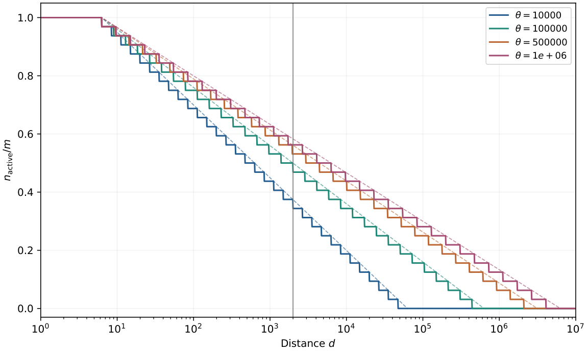
Uncycled fraction for \(m=32\) and four geometric bases. Solid curves use the exact integer count; dashed curves use the clipped continuous approximation. The vertical line marks \(d=2000\). The plotted quantities count phase thresholds and do not measure attention decay or a retrieval ceiling.
4.3 Three Reference Scales and the Exact Last-Cycle Distance
It is useful to retain three distinct reference scales, while separating their definitions. Only the first and third arise from the continuous count; the second is a chosen comparison coordinate.
↳ Not used by another result of the paper.
En palabras.
Las tres distancias son coordenadas de referencia distintas. \(2\pi \sqrt\theta \) y \(2\pi \theta \) vienen del recuento continuo; \(\theta /\sqrt2\) es una escala de comparación elegida. Para \(m\) finito, la última vuelta ocurre antes de \(2\pi \theta \).
Alcance.
Ninguna de estas distancias constituye por sí sola un límite de recuperación, de contexto útil o de compresión KV.
For integer \(1\le r{\lt}m\), exactly \(r\) planes are cycled on
For even \(m\), take \(r=m/2\) to obtain the exact half-count interval. At its upper endpoint \(2\pi \sqrt\theta \), one additional plane cycles. The final plane cycles at \(T_{\rm last}=2\pi \theta ^{(m-1)/m}\), before \(T_{\rm max}\). Thus neither endpoint is a proof that position becomes undetectable. Also, \(\theta /\sqrt2\) is not the zero of the Padé exponent in this paper: that candidate vanishes at \(T=\sqrt2\theta \).
|
\(\theta =10^4\) |
\(\theta =5\times 10^5\) |
\(\theta =10^6\) |
|
|
\(T_\mathrm {cross}\) |
628 |
4,443 |
6,283 |
|
\(d_\mathrm {alias}\) |
7,071 |
353,553 |
707,107 |
|
\(T_{\rm max}\) |
62,832 |
3,141,593 |
6,283,185 |
|
\(T_{\rm last}\) |
47,117 |
2,084,765 |
4,080,185 |
Colour: blue shade = the number’s size within its column.
Testing a common context scale.
Retrieval, context extension and cache compression investigate different observables liu2024lostinthemiddle,peng2023yarn,snapkv2024. A common dependence on \(\sqrt\theta \) would require matched experiments varying \(\theta \) while holding other factors fixed. The cycle count does not establish that these tasks share a context wall.
🖼️ Figure 3
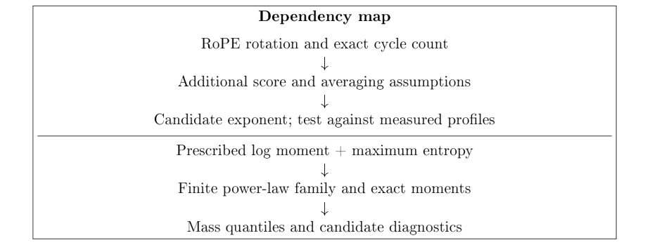
Logical dependencies. The MaxEnt branch starts from a prescribed constraint, not from the cycle count alone. Converting a mass quantile or an inverse parameter into a useful intervention requires separate empirical validation.
5 Modelling \(\gamma \): Geometry, Approximations and Empirical Tests
The rotary count is exact under its stated frequency schedule. A prediction for a trained attention exponent requires additional assumptions about content scores, normalization and aggregation. We develop the candidate construction explicitly, identify where those assumptions enter, and compare the result with saved measurements. The empirical fits do not prove the construction that motivated them.
5.1 The Empirical Starting Point
A power-law regression represents a sampled profile by
Here \(A(d)\) is a protocol-specific aggregate and \(\epsilon _d\) is its fitted log residual. The E4 program averages finite attention entries across heads and layers at the last query position, then across prompts and seeds. It discards non-finite entries without recording their final fraction. Random tokens change the content distribution; they do not remove learned content interactions or instrumental confounds. The October QL procedure instead has its own fixed-context profile and bootstrap protocol (Section 8).
The E4 panel contains both good and poor fits: for example, Pythia-1.4B text has \(R^2=.841258\), while Pythia-2.8B text has \(R^2=.999287\) on only three distances. Thus there is no supported statement that every tested model has \(R^2{\gt}.95\), or that every curve spans 10–2000. A descriptive power-law fit is not an exact law and does not uniquely identify its generative mechanism.
🖼️ Figure 4
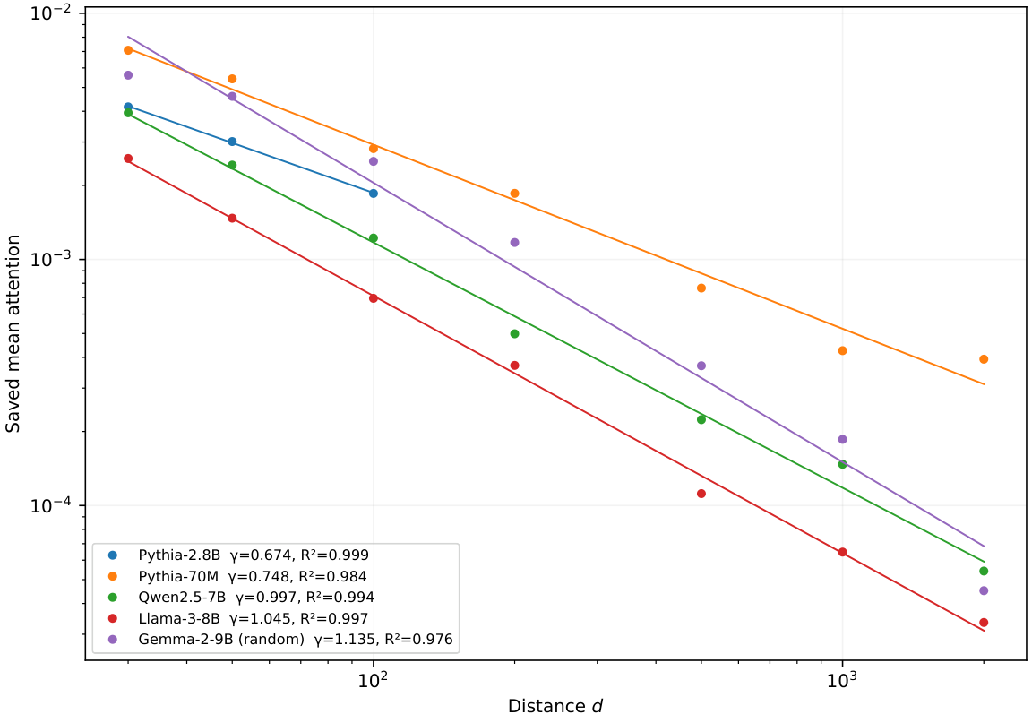
Five representative saved E4 profiles. Points are the means on each record’s declared fitting grid; lines use both slope and intercept from that regression. Pythia-2.8B covers only 30–100. The legend reports each actual \(R^2\); no uniform fit-quality claim is imposed.
5.2 From Rotary Coordinates to a Candidate Score
Groups 7–8 in Appendix K provide the verified score-to-softmax bound and the cosine-integral remainder under explicit row-level hypotheses.
Step 1: exact score decomposition.
Let \(\delta =n-m_0\) be the signed key-minus-query displacement, let \(h\) be the full head dimension, and let \(J=R'(0)\). For the \(m=d_{\rm rot}/2\) rotated pairs and the unrotated remainder \(q_\perp ,k_\perp \), the ordinary scaled dot-product score is
This follows by expanding \(R(\delta \omega _i)=I\cos (\delta \omega _i)+J\sin (\delta \omega _i)\) in each plane. Additional attention biases and masks must be added separately. In split-half implementations the physical coordinate pairing must match the implementation before applying this identity to weight rows.
Step 2: a conditional score model.
A cosine can already be negative before a full cycle: at phase \(\pi \) it equals \(-1\). Conversely, completing a cycle does not make its contribution average to zero over content. Small query/key covariance does not establish either assertion. An explicit modelling hypothesis would be
The coefficient \(a\) carries the amplitudes and score scaling; setting it to one is an additional choice. On the unclipped part of the continuous count this ansatz has a logarithmic distance term with coefficient \(-am/\log \theta \) and intercept \(b_1=b_0+am(1+\log (2\pi )/\log \theta )\).
Step 3: a conditional normalization model.
If an idealized row has deterministic scores \(b_1-\kappa \log d\) on a fixed support, then its softmax is exactly a power law:
Replacing random scores by their mean before softmax is not an identity. For equiprobable score vectors \((2,0)\) and \((0,0)\), the expected first softmax component is \(0.690399\), whereas the softmax of the mean gives \(0.731059\). Averaging across heads, query positions or contexts adds further noncommuting operations. In E4 the context length also changes with \(d\), so the normalization need not be the same across the plotted curve.
Pythia-70M has head dimension 64 but rotary dimension 16: its \(\texttt{rotary\_ pct}=0.25\) leaves only \(m=8\) rotated pairs. With \(a=1\) and \(\theta =10^4\), the conditional exponent is \(0.868589\), not \(3.474356\). Relative to the E4 text estimate \(0.747602\), the discrepancy is \(16.18\% \); the matched E4 uniform null is \(0.782582\). Correcting the dimension therefore does not validate the ansatz or its averaging assumptions. More directly, setting all query projections to zero gives uniform attention over unmasked keys for every RoPE base, provided no additional key-dependent score bias is present. That counterexample shows why RoPE geometry alone cannot force a nonzero power-law exponent.
A configuration check against fixed-query profiles.
Table 6 evaluates only the stipulated \(a=1\) ansatz, using \(m=d_{\rm rot}/2\) from saved configurations. The QL entries are the existing October text fits at \(T=2048\) in FP32. Every candidate lies outside its corresponding saved bootstrap interval. In particular, the two smallest rotary subspaces have the largest QL slopes in this six-row set; the slopes do not increase monotonically with \(m\) as this fixed-\(a\) candidate does. This is a descriptive negative check of that specification, not a controlled intervention on rotary dimension or a rejection of every learned score model. The 14M and 31M configurations were retrieved from the official model repositories with their resolved revisions; the other four are previously archived configs. These files do not retroactively certify the weight revisions of the October jobs.
|
Pythia |
\(d_{\rm rot}\) |
\(m\) |
\(\kappa =m/\log \theta \) |
QL [95% CI] |
|
14m |
8 |
4 |
0.434294 |
1.244245 [1.212552, 1.281474] |
|
31m |
8 |
4 |
0.434294 |
1.232606 [1.202567, 1.264370] |
|
70m |
16 |
8 |
0.868589 |
1.173706 [1.147172, 1.199493] |
|
1b |
64 |
32 |
3.474356 |
0.974251 [0.943375, 1.006482] |
|
1.4b |
32 |
16 |
1.737178 |
0.930250 [0.896514, 0.966649] |
|
2.8b |
20 |
10 |
1.085736 |
0.866809 [0.830561, 0.904920] |
Colour: blue shade = the number’s size within its column.
The score ansatz and the following rational candidate are different constructions. With a fixed alignment coefficient, \(\kappa =am/\log \theta \) depends on the rotary-pair count and has no context parameter; \(\gamma _P(\theta ,T)\) depends on context and omits that count. No identified relation between \(a,m,T\) connects them. The rational expression is a chosen configuration function, not a consequence of Steps 2–3.
A conditional cosine-integral alternative.
Writing \(S_m(d)=\sum _{i=0}^{m-1}\cos (d\theta ^{-i/m})\), its left Riemann approximation at fixed \(d,\theta {\gt}1\) is
For \(1\ll d\ll \theta \), the bracket is \(\log \theta -\gamma _E-\log d+O(d^{-1}+(d/\theta )^2)\). These are two distinct approximations. The absolute Riemann-sum error is bounded by the total variation, hence by \(d(1-1/\theta )\); this bound need not be small for a finite rotary subspace. The normalized error tends to zero as \(m\to \infty \) at fixed \(d,\theta \), not uniformly over arbitrary growing distance ranges. On 400 geometrically spaced distances from 10 to 2000, \(m=32\), \(\theta =10^4\), the fitted sum slope is \(-3.480436\) versus \(-m/\log \theta =-3.474356\), while the largest pointwise error against the integral is \(6.868580\). Agreement of fitted slopes alone does not control the individual oscillations.
If pre-RoPE plane dot products have a common, distance-independent mean \(a\), sine contributions have zero mean, and other score components have constant mean, the mean-score slope is conditionally \(-am/(\sqrt{d_{\rm head}}\log \theta )\). Here \(a\) is an unscaled plane dot product, unlike the score-scaled coefficient in Step 2. Measuring these amplitudes and the pre-softmax slope with fixed queries is a test of the assumptions. It does not commute expectation with softmax or derive the rational candidate.
Dimensionless candidate.
Define \(z=T\sqrt2/\theta \), using a chosen context parameter \(T{\gt}0\). The linear candidate is
The factor \(\sqrt2\) is part of this parametrization. It is not derived by the cycle count or by an asserted zero of a cosine sum at \(\theta /\sqrt2\). The actual half-count scale is discussed in Section 4.3. A negative exponent is mathematically admissible on finite support; whether it fits a particular observation is a separate question.
A finite cosine sum of the form
is not automatically a nonnegative normalized attention distribution. In particular, the proposed ratio of logarithms cannot supply the Padé exponent:
↳ Not used by another result of the paper.
For \(r{\gt}0\), \(\log (1/r)=-\log r\), and \(r\ne 1\) makes the denominator nonzero. Also \((2-z)/(2+z){\gt}-1\) for \(z{\gt}0\). A one-term cosine sum is negative when its phase is \(\pi \). These observations block the stated normalization and exponent inference. A stationary-phase argument would require an explicit asymptotic parameter, amplitude hypotheses and a controlled remainder; none is supplied by the finite sum alone.
En palabras.
Una suma finita de cosenos puede ser negativa y no define por sí sola una distribución de atención. Además, el cociente de logaritmos propuesto vale exactamente \(-1\) en su dominio, mientras que el candidato Padé es mayor que \(-1\) para \(z{\gt}0\). La proposición bloquea aquella derivación; no descarta que otra hipótesis sobre puntajes pueda producir una ley de potencias.
Alcance formal.
El paper da una prueba algebraica directa. Este enunciado completo no tiene un enlace Isabelle en este Blueprint.
🧪 Lab: Figure 5 live: turn the historical Padé candidate in 3D
Turn the candidate surface over log RoPE base and log context; the star marks your values. The flat curve below fixes your context. This stipulated formula is not inferred from the cosine sum or validated against a trained model.
5.3 The Padé Candidate and Its Domain
The rational candidate
is the \([1,1]\) Padé approximant to \(e^{-z}\) at zero, since both have expansion \(1-z+z^2/2+O(z^3)\). This local approximation theorem does not identify an observed exponent with \(e^{-z}\). For \(z{\gt}0\), \(-1{\lt}\gamma _P{\lt}1\); it is positive only for \(z{\lt}2\), vanishes at \(T=\sqrt2\theta \), and approaches \(-1\) as \(z\to \infty \). It therefore cannot predict observed exponents above one. Its derivatives describe the candidate function, not the response of trained weights to an intervention.
Approximation comparison.
The following are distinct candidate formulas, not successive increasing orders of one validated attention expansion:
The last function is \([0,1]\), with expansion \(1-z+z^2+O(z^3)\); it is not a higher-order approximation than \([1,1]\). For \(z{\gt}0\), its excess over \(\gamma _P\) is \(z^2/[(1+z)(2+z)]{\gt}0\). Selecting it after observing that an exponent exceeds \(\gamma _P\) uses the target to choose the predictor and does not establish prospective accuracy. Neither SWA nor GQA implies this correction. A context-window hypothesis must use the actual masking schedule and head/layer aggregation.
Implementation hypothesis.
A rational expression may be inexpensive to evaluate, but no gate is proved near-optimal by that fact. Routing quality, normalization, sparse-kernel cost and task error require direct benchmarking. The exponent parameter \(z=T\sqrt2/\theta \) must not silently become a per-distance kernel argument.
An algebraic shifted-base coordinate is
It gives the identity \(\gamma _P=1-T\sqrt2/\theta _{\rm eff}\) for this definition. It is not the base producing the same exponent at \(T=0\), since every positive base gives \(\gamma _P=1\) there. Nor is it the inverse fitted-base coordinate in Section 9; those are different definitions and cannot jointly diagnose training history.
|
Candidate |
Expression |
Relation to \(e^{-z}\) |
|
Linear |
\(1-z\) |
\([1,0]\); \(O(z^2)\) |
|
Exponential |
\(e^{-z}\) |
reference |
|
Padé |
\((2-z)/(2+z)\) |
\([1,1]\); \(O(z^3)\) |
|
Rational |
\(1/(1+z)\) |
\([0,1]\); \(O(z^2)\) |
|
Shorthand |
\(\log (10^4)/\log \theta \) |
no \(T\) dependence |
Colour: red = no / fails.
5.4 Initial-Panel Comparison with Explicit Inputs
Table 8 retains the 18 model/corpus entries of the initial predictor comparison, using the replayed exponents and bases actually recorded in their JSON files. Its set is P01–P21 excluding P02, P03 and P21; it includes P19 and P20 despite their missing base fields. This is different from the 18 stored-fit rows in Section 8, which exclude P02, P19 and P20. Five entries have no recorded base and therefore no computed candidate value here. For the remaining 13, \(T=2000\) is a stipulated comparison parameter; E4 acquisition itself used distance-dependent sequence lengths. The stored base fields are not a reconstruction of immutable model configurations. These limitations preclude treating this table as a controlled architectural experiment.
🖼️ Figure 5
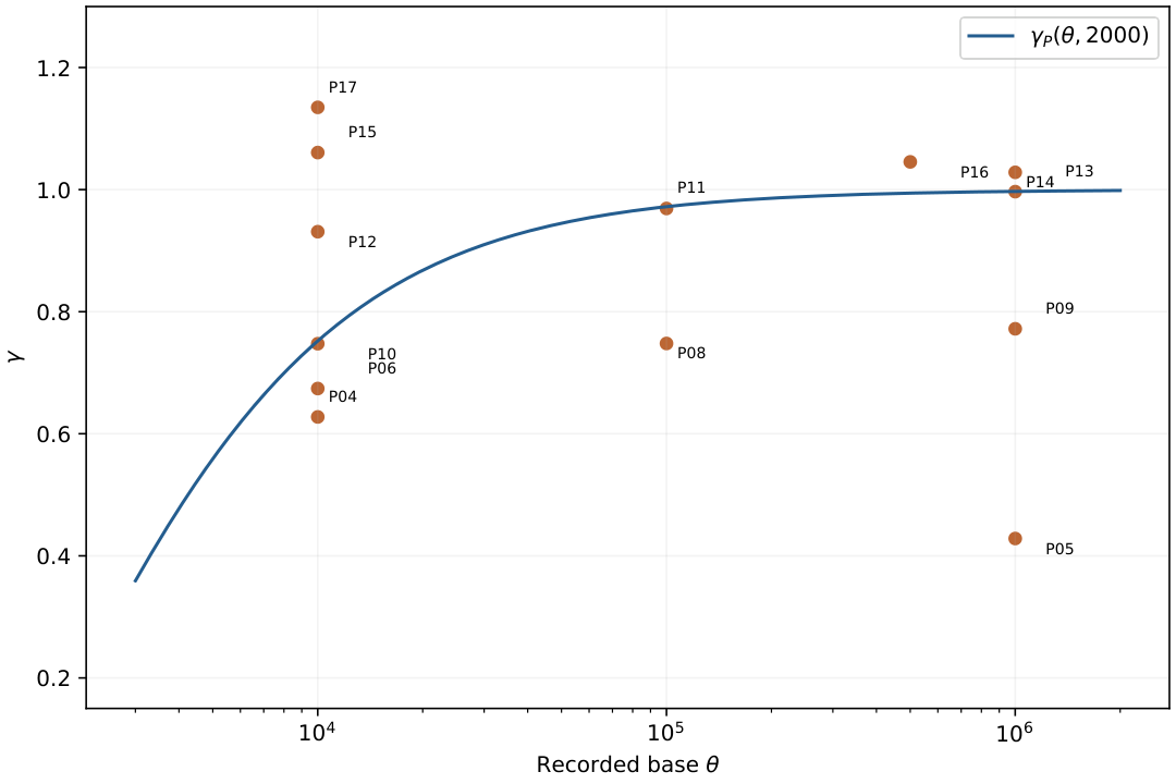
The candidate curve at stipulated \(T=2000\) and 13 observations with recorded base fields. Points use the same IDs as Table 8. A trend across different models is not an intervention on \(\theta \).
ID Model \(\theta \) \(\gamma _P\) \(\widehat\gamma \) \(R^2\) residual P01 phi-3-mini (text) — — 0.6296 0.9853 — P04 Gemma-2-9B (text) 10000 0.7522 0.6276 0.9773 -0.1246 P05 Mistral-Nemo-Instruct 1e+06 0.9972 0.4284 0.9224 -0.5687 P06 Pythia-2.8B 10000 0.7522 0.6742 0.9993 -0.0780 P07 Pythia-1.4B — — 0.7051 0.8413 — P08 SmolLM2-135M 100000 0.9721 0.7480 0.9889 -0.2241 P09 Qwen2.5-3B 1e+06 0.9972 0.7720 0.9958 -0.2251 P10 Pythia-70M 10000 0.7522 0.7476 0.9843 -0.0046 P11 SmolLM2-360M 100000 0.9721 0.9692 0.9981 -0.0029 P12 Pythia-1B 10000 0.7522 0.9311 0.9831 +0.1789 P13 Qwen2.5-7B 1e+06 0.9972 0.9967 0.9939 -0.0005 P14 Qwen2.5-0.5B 1e+06 0.9972 1.0284 0.9968 +0.0312 P15 Mistral-7B-v0.1 10000 0.7522 1.0608 0.9987 +0.3085 P16 Llama-3-8B 500000 0.9944 1.0455 0.9975 +0.0511 P17 Gemma-2-9B (random) 10000 0.7522 1.1348 0.9765 +0.3826 P18 phi-3-mini (random) — — 1.0366 0.9779 — P19 Llama-2-7B (Kaggle) — — 1.2108 0.9877 — P20 Llama-2-13B (Kaggle) — — 1.0545 0.9943 —
Colour: grey = nothing; blue shade = the number’s size within its column.
Unreconstructed selected-case statistic.
The earlier \(4.3\% \) median was attributed to nine selected “non-anomalous” cases. Neither an unambiguous nine-row membership list nor the selection and denominator calculation was recovered. The surviving Padé comparison JSON contains five entries and uses a prediction denominator; it does not establish the claimed nine-case statistic. We therefore withdraw that number as an accuracy result, rather than choose nine rows after observing their errors. The 13 identifiable comparisons here remain available in full, with the observed-exponent denominator stated above.
🖼️ Figure 6
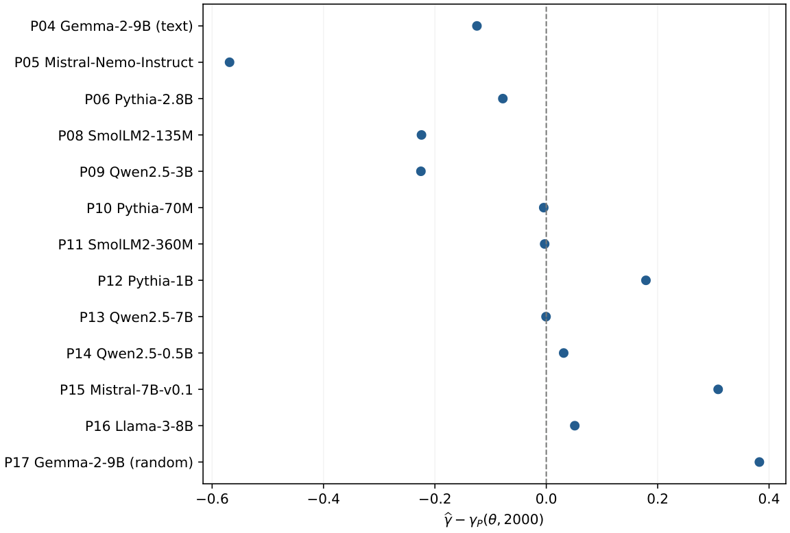
All 13 computable residuals, without excluding poorly predicted observations. Lack of fit is a limitation of the candidate; the residual alone does not identify its cause.
Across these 13 entries, mean absolute error is \(0.167766\), median absolute error \(0.124555\), and median absolute relative error \(19.2144\% \), using \(|\widehat\gamma |\) in the denominator. These are descriptive errors on a mixed initial panel, not an out-of-sample benchmark. The earlier selected-case percentages do not transfer to this denominator. In the separate October replay, only one historical text exponent lies in its corresponding interval among 25 observations, and the stored Padé comparison has rank correlation \(-0.445\) on 19 rows (Section 8).
Trivial predictors on the same 13 rows.
The mean absolute errors are \(0.182656\) for the constant one, \(0.177669\) for the panel mean and \(0.172106\) for the panel median, compared with \(0.167766\) for \(\gamma _P\). The latter improves on the median by only \(0.004340\) (about \(2.52\% \)). The mean and median use this same panel, so this is an in-sample descriptive comparison, not a held-out baseline experiment or proof of zero predictive information. Prospective usefulness has not been demonstrated. Adding present-day public bases to the five missing fields would be a separate imputation analysis; it would not recover the configurations of those historical executions.
Across-model base comparison.
The five entries below retain the original comparison across three nominal base scales. They vary in model size, training, corpus handling and support; they are not a controlled \(\theta \) sweep. A genuine test would modify only the frequency schedule in the same model under matched measurement conditions, and distinguish inference-time changes from retraining.
|
ID |
\(\theta \) |
\(\gamma _P\) |
\(\widehat\gamma \) |
|
P10 |
10000 |
0.752201 |
0.747602 |
|
P06 |
10000 |
0.752201 |
0.674162 |
|
P11 |
100000 |
0.972110 |
0.969173 |
|
P14 |
1e+06 |
0.997176 |
1.028374 |
|
P13 |
1e+06 |
0.997176 |
0.996695 |
Colour: blue shade = the number’s size within its column.
5.5 Exploratory Five-Axis Regression
The original exploratory specification regresses the text exponent on five covariates:
The source script supplies manual architecture flags, a \(T=100\) candidate parameter, and a size-derived “post-IH” flag; the latter is not a measured circuit label. Replaying its 23-row design matrix reproduces the following coefficients. This is a check of the original regression specification, not an endorsement of its metadata or identification assumptions.
|
Coefficient |
Estimate |
|
\(\beta _0\) |
+4.578763 |
|
\(\beta _P\) |
-3.686409 |
|
\(\beta _c\) |
+0.597427 |
|
\(\beta _G\) |
+0.107691 |
|
\(\beta _S\) |
+0.001117 |
|
\(\beta _{\rm IH}\) |
-0.151244 |
The fit has \(R^2=0.437821\), adjusted \(R^2=0.272474\), and residual standard deviation \(0.164644\). The corpus covariate contains the response \(\widehat\gamma _t\) itself, so the regression is not a configuration-only predictor and its apparent explanatory power can include target leakage. The near-constant Padé column is also nearly collinear with the intercept. A ratio of predictor variance to observed variance is not variance explained; unexplained variance cannot automatically be assigned to the other axes.
The largest original-specification residuals are approximately \(+.47\) (Pythia-31M), \(-.33\) (SmolLM2-135M), \(-.26\) (OLMo-7B), \(-.19\) (Pythia-2.8B) and \(-.18\) (Llama-2-7B). They motivate tests of tokenization, data, optimization and measurement support but do not identify these factors. In particular, the unequal-support Pythia-2.8B corpus contrast needs the correction in Section 8.4.
A useful hypothesis notation remains
Without interventions or identifying restrictions, infinitely many assignments of the \(\delta \) terms give the same residual. The decomposition does not establish a geometric ceiling, a fixed median, or that the perturbations explain \(99\% \) of variance. Measured exponents above one already exceed the positive-\(z\) range of \(\gamma _P\).
5.6 Derived Quantities and Testable Consequences
P1: entropy conditional on the family.
For the finite family, the identity is
The entropy columns in the initial thermodynamic dataset were derived from fitted exponents; they are not independent entropy observations. A test must instead measure a normalized empirical distribution on the same support and compare its entropy with the fitted-family value, accounting for estimation uncertainty. Normalizing values at seven sampled distances gives the entropy of a seven-point variable, which cannot be directly equated with entropy over 2000 token distances.
P2: entropy-based effective count.
The exponential of Shannon entropy is
The product uses probability weights \(p_\gamma (d)\), not uniform weights \(1/N\). For \(N=2000\), exact finite sums give \(N_{\rm eff}=1160.379\) at \(\gamma =.65\) and \(362.107\) at \(.95\). For fixed \(0{\lt}\gamma {\lt}1\), \(N_{\rm eff}/N\to e^{-\gamma /(1-\gamma )}/(1-\gamma )\); for fixed \(\gamma {\gt}1\), \(N_{\rm eff}\) tends to a finite constant and \(N_{\rm eff}/N\to 0\). These are diversity measures of the chosen distance distribution. They do not bound multi-hop reasoning spans, factuality or the number of useful tokens in a trained network.
P3: layer variation with missing fits reported.
We recompute layer means from finite entries of the saved per-head exponent matrices, exclude the actual first and last architecture layers, and report the population standard deviation across the remaining observed layer means. Entirely missing interior layers remain missing; they are not reclassified as boundary layers. Some observed layers also lack individual head fits, as recorded in the evidence manifest.
|
Model |
observed |
missing |
mean |
std |
CV |
|
pythia-70m |
3 |
1 |
1.424844 |
0.248423 |
0.174351 |
|
pythia-410m |
14 |
8 |
1.309708 |
0.175708 |
0.134158 |
|
pythia-1b |
14 |
0 |
0.915502 |
0.137759 |
0.150474 |
|
pythia-1.4b |
22 |
0 |
0.900704 |
0.231879 |
0.257442 |
|
pythia-2.8b |
30 |
0 |
1.326845 |
0.257319 |
0.193933 |
Colour: blue shade = the number’s size within its column.
Four of five available-case summaries have \(\mathrm{CV}{\lt}.20\), and only one has \(\mathrm{CV}{\lt}.15\). Pythia-1.4B has \(\mathrm{CV}=.257442\). The data do not establish a universal layer-stability bound or a geometric cause. In particular, partial matrices cannot certify whole-model stability. The former procedure removed the last observed layer after filtering missing layers, which need not remove the architectural boundary.
P4: short- and long-distance residuals.
Flattening at short distance and faster decay at long distance are testable candidate patterns. They are not consequences of “all planes uncycled below \(2\pi \sqrt\theta \)”, which is false: the first threshold is \(2\pi \). Training length also does not force every phase to alias uniformly. The saved BLOOM-1b7 extended-distance record contains a numerical zero at \(d=5000\), with non-monotonic positive values at 2048 and 3000. A numerical zero in one ALiBi experiment is not a theorem about RoPE or proof of a universal hard cutoff. Testing residual signs requires a predeclared fitting interval, actual training context and adequate positive observations in each region.
Null baselines on the available saved fits.
We compare power-law and exponential regressions in log-attention space on each record’s declared distance grid, using canonical text/random files with at least three positive points and a stored fit. The resulting set has 74 profiles, of which 72 favor the power law by in-sample \(R^2\); the median difference is \(+.203803\). The manifest lists every included record. This is a descriptive model-form comparison, with unequal ranges and no held-out evaluation. It does not rule out mixtures, content-dependent mechanisms, or learned-only explanations, and it does not prove a MaxEnt constraint. Correlation across architectures cannot exclude training or data as a cause.
6 Why Power Law: The Maximum Entropy Foundation
The finite power-law family follows from a specified entropy-maximization problem. The constraint and the reference measure are premises of that problem. RoPE’s frequency geometry does not establish that a trained attention distribution solves it. This section supplies the conditional mathematical result and its connection to measured profiles.
Let \(N\ge 1\) be an integer and \(\gamma \in \mathbb R\). Define
Among all probability vectors \(p\) on this support satisfying \(\mathbb E_p[\log d]=\mathbb E_{p_\gamma }[\log d]\), the unique entropy maximizer is \(p_\gamma \). We use counting measure, natural logarithms and \(0\log 0=0\).
Lean · ours, in partshow
Lean demuestra la desigualdad y la igualdad de Gibbs para la familia finita; el enunciado del paper permite cualquier exponente real y N=1, mientras el fichero Lean enlazado trata N>0 y el resultado de existencia se formula para exponente positivo.
✅ Checked when this page was built: MaxEnt.lean compiles with Lean 4.35.0, no errors, no sorry. Axioms — gibbs_le: propext, Classical.choice, Quot.sound.
Reproduce: Lean 4.35.0, Mathlib f0b4c8150aa0; in that Lean project, lake env lean MaxEnt.lean (SHA-256 of the compiled file: 5d78934b6d41f005…; a source page on this site may show it with comments edited, under its own hash).
Trust base: 🔒 kernel only — only part of the statement is formal (see the box). Lean: 1 result, standard axioms only
Cite: Definition 4.1, p. 15, doi:10.5281/zenodo.24379538
🆕 Classical and new: Resultado clásico de máxima entropía con una restricción prescrita; no prueba una ley de entrenamiento.
↳ Used in: Theorem 6.2
The reference vector is strictly positive. Since \(\log p_\gamma (d)=-\gamma \log d-\log Z_N\), the moment and normalization constraints give \(\sum p\log p_\gamma =\sum p_\gamma \log p_\gamma \). Consequently,
Gibbs’ inequality applies also when some entries of \(p\) vanish. Equality holds only for \(p=p_\gamma \). This proves global optimality and uniqueness, rather than only a stationary point of a Lagrangian.
En palabras.
En un soporte finito, si se fija la media de \(\log d\) al valor de una familia de potencias dada, esa familia maximiza de forma única la entropía. La prueba compara la entropía mediante divergencia KL y usa su no negatividad. El momento fijado es una premisa matemática, no una consecuencia de RoPE ni del entrenamiento de un modelo.
Alcance formal.
El argumento está escrito en el paper. Lean verifica la desigualdad de Gibbs para la familia finita; el enunciado completo para todo exponente y \(N=1\) mantiene aquí una prueba escrita, sin certificado formal de igual alcance.
[colback=ModernTint,colframe=ModernTeal,title=What the constraint does and does not select,fontupper=] Exponential, Gaussian-shaped or cutoff distributions on a finite set can have the same log-distance moment. They are not excluded as empirical models of attention. The theorem singles out the entropy maximizer among feasible distributions. Competing profile families must be compared on the same observations, support and loss; differentiability in distance is not required on a discrete support.
Example: a six-sided die. If the only prescribed statistic is the average of \(\log (\mathrm{face})\), choosing maximum entropy assigns \(p(k)\propto k^{-\gamma }\) on \(\{ 1,\ldots ,6\} \). This is an inference rule under limited information. It does not establish that a physical loaded die, or a trained transformer, must realize that rule.
6.1 The MaxEnt Problem
For integer \(N{\gt}1\) and \(0{\lt}\lambda {\lt}\log N\), consider
There is a unique real exponent and a unique maximizing distribution:
The exponent is positive, zero or negative according as \(\lambda \) is below, equal to or above \(\log (N!)/N\). At the endpoints \(\lambda =0\) and \(\lambda =\log N\), the feasible distribution is the point mass at \(1\) or \(N\), respectively, obtained as an exponent limit. For \(N=1\) the distribution is unique but the exponent is unidentifiable.
Lean · ours, in partshow
Lean certifica existencia, unicidad y máximo para 0<lambda<log(N!)/N, con exponente positivo. El paper también afirma los regímenes de exponente cero y negativo y los extremos; esas partes quedan fuera de estos teoremas Lean.
✅ Checked when this page was built: MaxEnt.lean compiles with Lean 4.35.0, no errors, no sorry. Axioms — maxent_power_law, gamma_unique: propext, Classical.choice, Quot.sound.
Reproduce: Lean 4.35.0, Mathlib f0b4c8150aa0; in that Lean project, lake env lean MaxEnt.lean (SHA-256 of the compiled file: 5d78934b6d41f005…; a source page on this site may show it with comments edited, under its own hash).
Trust base: 🔒 kernel only — only part of the statement is formal (see the box). Lean: 2 results, standard axioms only
Proof: in this note·Formalized: Lean 4, by the author (public formalizations repository)·Covers: part: Lean certifica existencia, unicidad y máximo para 0<lambda<log(N!)/N, con exponente positivo. El paper también afirma los regímenes de exponente cero y negativo y los extremos; esas partes quedan fuera de estos teoremas Lean.·Cite: Theorem 6.2, p. 28, doi:10.5281/zenodo.24379538
🆕 Classical and new: Aplicación explícita de Gibbs y del orden estricto del momento; resultado matemático condicional.
↳ Not used by another result of the paper.
The Lagrangian \(\mathcal L=H(p)-\mu (\sum p-1)-\gamma (\sum p\log d-\lambda )\) has stationary equation \(-\log p(d)-1-\mu -\gamma \log d=0\). Normalization gives the displayed family. To establish existence of the required exponent, define \(U_N(\gamma )=\mathbb E_{p_\gamma }[\log d]\). Finite-sum differentiation gives
Strict negativity follows because all probabilities are positive and \(\log d\) is nonconstant for \(N{\gt}1\). As \(\gamma \to +\infty \), mass concentrates at \(1\) and \(U_N\to 0\); as \(\gamma \to -\infty \), it concentrates at \(N\) and \(U_N\to \log N\). Continuity and strict monotonicity establish existence, uniqueness and the sign condition. The preceding Gibbs argument then proves global optimality over all feasible vectors, including their boundary.
En palabras.
Para un momento logdistancia interior, existe exactamente un exponente de la familia finita que lo realiza. La derivada del momento es menos una varianza estrictamente positiva, lo que da el orden y la unicidad; el argumento de Gibbs del teorema precedente da la optimalidad global. Los extremos requieren límites de exponentes y, si \(N=1\), el exponente no se puede identificar.
Alcance formal.
Lean verifica existencia, unicidad y óptimo para el momento interior que da exponente positivo. Los regímenes de exponente cero o negativo y los extremos del enunciado completo siguen demostrados en el manuscrito.
Interpretation
The theorem is a constrained inference result, not a training-dynamics result. Its premise must be justified separately when the family is applied to attention. Models with identical RoPE configuration can learn different queries and keys and produce different profiles. The exploratory five-axis panel in Section 5.5 reports a population residual standard deviation \(0.164644\) (approximately \(0.16\)) in its exploratory multiple regression, not a measured variance at fixed configuration; neither that regression nor an assumed centroid turns the MaxEnt premise into a geometric necessity.
6.2 Thermodynamic Interpretation
The family can be written in Gibbs form:
This is a mathematical dictionary for a chosen probability family. The inverse-temperature coordinate is not the output sampling temperature, and the dictionary alone does not identify a physical equilibrium process or a trained model’s response to an intervention.
|
Quantity |
Formula |
Scope |
|
Inverse temperature |
\(\gamma \) |
Family parameter, not a measured physical temperature. |
|
Temperature |
\(1/\gamma \) |
Defined for \(\gamma \ne 0\); increasing positive \(\gamma \) favors shorter distances. |
|
Partition function |
\(\sum _{d=1}^N d^{-\gamma }\) |
Finite for every finite \(N\); the infinite sum converges only for \(\gamma {\gt}1\). |
|
Heat capacity |
\(-\gamma ^2 U_N'(\gamma )\) |
A finite-family susceptibility, not task sensitivity. |
For \(S=\log Z_N+\gamma U_N\), differentiation cancels the two terms involving \(U_N\) alone. Since \(U_N'{\lt}0\) for \(N{\gt}1\), the parameterization gives
6.3 Duality with Zipf’s Law
Zipf’s vocabulary law zipf1949human and a distance power law can both be represented by constrained-entropy families. For two members of the same finite power-law family with integer \(N{\gt}1\), strict monotonicity of its log moment identifies equal exponents. This requires the same support and reference measure and the family assumption:
Vocabulary ranks and token distances generally have different supports. The seven successful saved pairs give \(r(\alpha _{\rm Zipf},\gamma )=-0.505314\). No corrected positive correlation is established. The three Pythia rows have constant rank exponent, so their within-group Pearson correlation is undefined (Appendix D).
6.4 Finite Thermodynamic Functions
Group 5 in Appendix K gives the full smoothness, entropy and divergence statements for this finite family, with proofs.
The discrete quantities are defined by exact sums: [nobreak=true]
Separately, with Lebesgue measure on \([1,N]\), the continuous normalizer is
The continuous and discrete moments must not be mixed. A tail fit on \([16,T/2]\) does not establish this family over all of \([1,N]\). The support and whether a quantity is measured or calculated from an exponent accompany each application.
Derived numerical examples
At \(N=2000\), using the full-precision replayed exponents of P10, P06, P13, P16 and P17, respectively, the family heat capacities are \(2.5396\), \(1.8335\), \(5.4488\), \(5.9361\) and \(6.5951\). These are the same inputs and rounding convention as Section 8. The discrete maximum is near \(\gamma =1.256885\), with \(C_V=6.919812\). These are calculations for the stipulated family, not moments measured from model attention rows.
7 Finite Power-Law Families and Infinite-Support Limits
7.1 The Partition Function and Phase Structure
For a fixed real exponent, the infinite-support limit of the discrete normalizer distinguishes three summability regimes:
Every finite-\(N\) distribution remains normalized. Divergence of the unnormalized infinite sum means that the same weights cannot be normalized on all positive integers; it does not mean a model has infinite attention mass or unbounded retrieval ability. For \(\gamma {\gt}1\) the limiting distribution still has an infinite tail, not a hard finite horizon. The term Hagedorn hagedorn1965statistical denotes an analogy to a summability boundary, not an identification with a physical phase transition. Analogy and its limit. A change of regime can be pictured as a phase boundary. Unlike a boiling or freezing system, however, the finite sums here are analytic functions of \(\gamma \). The mathematical limit \(N\to \infty \) must be distinguished from an intervention on a finite-context network.
7.2 Continuous and Discrete Heat Capacity at One
Let \(N{\gt}1\) and let \(p_c(x)=1/(x\log N)\) be a probability density on \([1,N]\) with respect to Lebesgue measure. Then
Lean · ours, in partshow
Lean comprueba la identidad algebraica L²/3−(L/2)²=L²/12; la transformación de la densidad continua a uniforme y el cálculo de los dos momentos siguen demostrados en el texto.
✅ Checked when this page was built: HeatCapacity.lean compiles with Lean 4.35.0, no errors, no sorry. Axioms — var_log_d_identity: propext, Classical.choice, Quot.sound.
Reproduce: Lean 4.35.0, Mathlib f0b4c8150aa0; in that Lean project, lake env lean HeatCapacity.lean (SHA-256 of the compiled file: b9789e37fc15f362…; a source page on this site may show it with comments edited, under its own hash).
Trust base: 🔒 kernel only — only part of the statement is formal (see the box). Lean: 1 result, standard axioms only
Proof: in this note·Formalized: Lean 4, by the author (public formalizations repository)·Covers: part: Lean comprueba la identidad algebraica L²/3−(L/2)²=L²/12; la transformación de la densidad continua a uniforme y el cálculo de los dos momentos siguen demostrados en el texto.·Cite: Theorem 7.1, p. 31, doi:10.5281/zenodo.24379538
↳ Not used by another result of the paper.
Write \(L=\log N\). The change of variable \(y=\log x\), with \(\mathrm dy=\mathrm dx/x\), maps the density to the uniform distribution on \([0,L]\). Direct integration gives
Subtracting the square of the first moment from the second gives \(L^2/3-L^2/4=L^2/12\). This calculation concerns the continuous density, not harmonic probabilities on integer distances.
En palabras.
Para la densidad continua \(1/(x\log N)\), el cambio \(y=\log x\) produce una uniforme en \([0,\log N]\). Su varianza es \((\log N)^2/12\). Esta cuenta continua difiere de la varianza de las distancias enteras y no establece una transición de fase en un transformer.
Alcance formal.
Lean verifica la identidad algebraica de los dos momentos. La transformación de la densidad y las integrales continuas se demuestran en el manuscrito.
Equivalent continuous expansion
For \(\epsilon =1-\gamma \) and fixed \(L\), \(Z_c=(e^{\epsilon L}-1)/\epsilon \) has a removable singularity at zero. Its analytic expansion gives
Taking the derivative at \(\epsilon =0\) recovers the same variance. The remainder terms are essential: a truncated expansion is not an exact expression for \(U_c\) away from one, and a first-order normalizer is insufficient for its second derivative.
For discrete token distances, the exact value instead is
At \(N=2000\), the continuous value is \(4.81448\), while the discrete value is \(5.48412\). Finite-sum calculation places the discrete maximum near \(\gamma =1.256885\), with \(C_V=6.919812\). Both remain finite. These numbers are derived family calculations, not independent measurements on language models.
7.3 Fisher Information and Heat Capacity
On fixed finite support, \(\partial _\gamma \log p_\gamma (d)=U_N-\log d\). Squaring and averaging therefore gives
At \(\gamma =0\), \(I\) is evaluated directly as a variance; division by \(\gamma ^2\) is not defined. Neither quantity is singular at finite \(N\). Their extrema need not coincide because \(C_V'=2\gamma I+\gamma ^2 I'\). For \(N{\gt}1\), the intrinsic Fisher length inside this one-parameter family is
The integral uses \(\sqrt I\), not \(I\). This is a distance along the specified statistical family; it is not automatically the ambient simplex geodesic or a distance between trained networks with different protocols.
7.4 Finite Entropy Bound and Asymptotic Regimes
For integer \(N{\gt}1\) and the discrete family \(p_\gamma \), define \(S_\gamma (N)=-\sum p_\gamma \log p_\gamma \).
For every real \(\gamma \), \(0\le S_\gamma (N)\le \log N\), with equality in the upper bound exactly at \(\gamma =0\). For \(N=1\) the entropy is zero for every exponent.
For fixed \(0{\lt}\gamma {\lt}1\), as \(N\to \infty \),
\begin{equation} S_\gamma (N)=\log N-\log (1-\gamma )-\frac{\gamma }{1-\gamma } +O(N^{\gamma -1}\log N). \end{equation}40At \(\gamma =1\), \(S_1(N)=\tfrac 12\log N+\log \log N-\gamma _E/2+o(1)\). This is a separate asymptotic regime, not substitution into the preceding fixed-exponent formula.
For fixed \(\gamma {\gt}1\), \(S_\gamma (N)\to \log \zeta (\gamma )-\gamma \zeta '(\gamma )/\zeta (\gamma ){\lt}\infty \).
Lean · ours, in partshow
Lean demuestra la cota superior finita y su caso de igualdad para distribuciones en un alfabeto finito; los tres regímenes asintóticos del teorema no están formalizados ahí.
✅ Checked when this page was built: EntropyBound.lean compiles with Lean 4.35.0, no errors, no sorry. Axioms — entropy_le_log_card, entropy_eq_log_card_iff: propext, Classical.choice, Quot.sound.
Reproduce: Lean 4.35.0, Mathlib f0b4c8150aa0; in that Lean project, lake env lean EntropyBound.lean (SHA-256 of the compiled file: e0abf82c9a53cede…; a source page on this site may show it with comments edited, under its own hash).
Trust base: 🔒 kernel only — only part of the statement is formal (see the box). Lean: 2 results, standard axioms only
Proof: in this note·Formalized: Lean 4, by the author (public formalizations repository)·Covers: part: Lean demuestra la cota superior finita y su caso de igualdad para distribuciones en un alfabeto finito; los tres regímenes asintóticos del teorema no están formalizados ahí.·Cite: Theorem 7.2, p. 32, doi:10.5281/zenodo.24379538
↳ Not used by another result of the paper.
The first part is the finite-alphabet Shannon bound, with equality only at the uniform vector. For \(N{\gt}1\), the power-law vector is uniform exactly when \(\gamma =0\). For the second part, integral comparison (or Euler–Maclaurin with fixed exponent) gives \(Z_N=N^{1-\gamma }/(1-\gamma )+O(1)\) and \(U_N=\log N-1/(1-\gamma )+O(N^{\gamma -1}\log N)\). Substitute into \(S=\log Z_N+\gamma U_N\). At one, \(H_N=\log N+\gamma _E+O(N^{-1})\) and \(\sum _{d\le N}\log d/d=\tfrac 12(\log N)^2+O(1)\) yield the stated separate expansion. Above one, both \(\sum d^{-\gamma }\) and \(\sum d^{-\gamma }\log d\) converge, giving the zeta expression. The fixed-exponent remainder bounds are not uniform as \(\gamma \to 1\).
En palabras.
La entropía de una distribución sobre \(N\) distancias no supera \(\log N\). La familia de potencias tiene además tres regímenes asintóticos distintos: exponente fijo menor que uno, igual a uno y mayor que uno. La fórmula del primer régimen no se puede sustituir directamente en uno porque su resto no es uniforme al acercarse a ese punto.
Alcance formal.
Lean verifica la cota finita y su igualdad uniforme; las tres expansiones asintóticas se demuestran en el manuscrito. Ninguna es una medición de modelos.
Calculated model-panel quantities
For the 21 initial-panel model/corpus entries in Section 8, exact finite-family entropies at \(N=2000\) range from \(4.377455\) to \(7.477491\). Each value is calculated from the corresponding replayed exponent, not independently measured from attention. Their association with \(\gamma \) cannot validate the finite-alphabet theorem or a physical mechanism. The table reports the input exponents and the derived values together.
Scope of the holographic analogy
The Ryu–Takayanagi relation ryu2006holographic concerns entanglement entropy and geometric areas in its stated physical setting. A logarithmic Shannon bound for a distance variable establishes neither that setting nor a central charge \(c=3\). Matching its leading coefficient to a CFT formula is insufficient. Likewise, the bound does not create thermodynamic pressure that reallocates rotary coordinates to semantic content. Such a channel interpretation requires separate functional evidence. Work on learning inverse holographic maps jhep2026rttransformer concerns a different learning problem and does not identify the operator or geometry of the models studied here.
Threshold-count exponent \(1/\gamma \)
For the normalized family, a probability threshold has the finite-support count
The notation \(d_{\rm eff}\) records an exponent of threshold scaling, not a Hausdorff or box-counting dimension of model states. The unnormalized weights \(d^{-\gamma }\) give \(\lfloor \epsilon ^{-1/\gamma }\rfloor \) before clipping to \(N\). The examples \(\gamma =.674\) and \(1.045\) yield \(1/\gamma \approx 1.48\) and \(0.96\), respectively; at one the reciprocal is one. These arithmetic values do not prove a fractal support, measure-zero addressability or exclusion of hyperbolic architectures such as Hypformer chen2024hypformer. Measuring a geometric dimension of per-head support is a separate proposed experiment.
Band ablation measurements in EXP-B3
The full saved window sweep and exact mask audit are in Section 13, Table 24. The historical groups are unequal adjacent-coordinate masks rather than two sets of intact rotary planes. The larger mask has higher PPL at every saved window. Neither the finite entropy bound nor those ablations establish a semantic reservoir or a semantic/positional double dissociation. The schematic has been replaced by the recorded PPL curves in Figure 13.
7.5 The Family with an Exponential Cutoff
A second family adds a cutoff coefficient \(\lambda \ge 0\); here \(\lambda \) is distinct from the prescribed log moment in Section 6. Its infinite-support normalizer, when convergent, is
At \(\lambda =0,\gamma =1\), \(Z_N=H_N\sim \log N\). The other cases are
↳ Not used by another result of the paper.
En palabras.
La definición clasifica cuándo converge el normalizador de una familia de potencias con posible corte exponencial en soporte infinito. Con corte positivo converge para todo exponente; sin corte, el umbral de sumabilidad está en uno.
Alcance.
Son casos de una distribución matemática. No clasifican automáticamente arquitecturas ni prueban una transición de fase en modelos entrenados.
These are distributional cases, not an automatic partition of architectures. An ALiBi bias may motivate an exponential positional factor, but learned content scores also contribute. The reported mean distances of 19 tokens for BLOOM and 772 for Falcon remain panel observations; they are not implied by the normalizer alone.
Exploratory size regression
The previously printed expression is retained only to identify the withdrawn claim:
With \(N_{\rm params}\) in individual parameters, it gives \(3.153474\) at 14M and \(1.930059\) at 7B, incompatible with the panel it was said to describe. Keeping the coefficient fixed while expressing counts in millions or billions makes these predictions larger, not smaller. No source fit, row manifest or declared alternative normalization was recovered to repair the coefficient or exponent; the accompanying \(R^2=0.41\) is therefore withdrawn too. The available E9 script concerns eight Pythia sizes, and its saved log reports zero parsed observations, not a successful 16-model fit. A new fit to an explicit panel would be a new analysis and is not silently substituted here.
8 Protocol-Specific Exponents and Derived Family Coordinates
This section distinguishes measured distance profiles, regression estimates, and quantities calculated from a fitted distribution. The initial E4 records and the October QL atlas use different acquisition and aggregation protocols. Each is analysed on its own support. Agreement between them is an empirical question, not a consequence of the finite-family identities.
8.1 Initial E4 Panel: Data and Regression Protocol
The matched uniform null for this extractor is nonflat. The 21 original rows below remain the recorded observable. Table 10 now shows the uniform null and excess slope on each row’s own grid, also supplied in the accompanying CSV. These are instrument diagnostics, not new measurements or an unbiased decomposition into learned and geometric effects. See Section 9.1 for the instrument test and its limits.
The saved records contain mean attention at sampled distances, usually with three seed means. For a declared fitting grid \(D\), we regress \(\log A(d)\) on \(\log d\) with an intercept and equal weight per distance. The slope with reversed sign is \(\widehat\gamma \). We use the exact saved grid when available. For the partial Falcon record and the two Kaggle Llama-2 records, which contain no fitting grid, the present analysis explicitly uses all saved distances \(d\ge 30\). These are recomputed estimates from those aggregates; they do not reconstruct an undocumented original fit.
The source measurement program uses sequences of length \(d+50\) at each distance, rather than one fixed context for the entire curve. Its text mode draws from the MongoDB episode corpus and its random mode generates token sequences. Complete records generally list seeds 42, 123 and 7 and a nominal prompt count of 150. The program can use a different prompt count at large distances, but that option is not recorded in the final JSON. Consequently, 150 must not be asserted as the verified count at every distance or as 150 independent prompts pooled across all seeds. The saved aggregates do not establish the exact corpus snapshot, immutable weight revision, loading precision, or correspondence of prompts between corpora.
For the 18 rows with a stored power-law estimate, the replayed exponent agrees within \(8\times 10^{-16}\). This verifies regression arithmetic on the saved inputs; it does not validate attention instrumentation or the acquisition of those inputs. No new model inference is performed. The accompanying evidence manifest maps P01–P21 to input paths and SHA-256 hashes, preserves the previous printed values, and records sensitivity to lower distance cutoffs 10, 30 and 50.
8.2 Complete Initial Panel: 21 Model/Corpus Entries
|
ID |
Model |
\(\widehat\gamma \) |
\(R^2\) |
Range / \(n\) |
\(\widehat\gamma _0\) |
excess |
|
P01 |
phi-3-mini (text) |
0.629563 |
0.985314 |
30–1000 / 6 |
0.741726 |
-0.112163 |
|
P02 |
Falcon-7B |
0.924685 |
0.989728 |
30–1000 / 6 |
0.741726 |
+0.182958 |
|
P03 |
CodeLlama-13B |
0.382302 |
0.928789 |
30–2000 / 7 |
0.782582 |
-0.400280 |
|
P04 |
Gemma-2-9B (text) |
0.627646 |
0.977314 |
30–2000 / 7 |
0.782582 |
-0.154936 |
|
P05 |
Mistral-Nemo-Instruct |
0.428448 |
0.922354 |
20–1000 / 7 |
0.698299 |
-0.269851 |
|
P06 |
Pythia-2.8B |
0.674162 |
0.999287 |
30–100 / 3 |
0.525737 |
+0.148425 |
|
P07 |
Pythia-1.4B |
0.705073 |
0.841258 |
30–2000 / 7 |
0.782582 |
-0.077510 |
|
P08 |
SmolLM2-135M |
0.747996 |
0.988937 |
30–2000 / 7 |
0.782582 |
-0.034586 |
|
P09 |
Qwen2.5-3B |
0.772033 |
0.995841 |
30–2000 / 7 |
0.782582 |
-0.010549 |
|
P10 |
Pythia-70M |
0.747602 |
0.984269 |
30–2000 / 7 |
0.782582 |
-0.034981 |
|
P11 |
SmolLM2-360M |
0.969173 |
0.998139 |
30–2000 / 7 |
0.782582 |
+0.186590 |
|
P12 |
Pythia-1B |
0.931108 |
0.983104 |
30–2000 / 7 |
0.782582 |
+0.148526 |
|
P13 |
Qwen2.5-7B |
0.996695 |
0.993942 |
30–2000 / 7 |
0.782582 |
+0.214113 |
|
P14 |
Qwen2.5-0.5B |
1.028374 |
0.996775 |
30–2000 / 7 |
0.782582 |
+0.245792 |
|
P15 |
Mistral-7B-v0.1 |
1.060750 |
0.998690 |
30–2000 / 7 |
0.782582 |
+0.278168 |
|
P16 |
Llama-3-8B |
1.045476 |
0.997461 |
30–2000 / 7 |
0.782582 |
+0.262894 |
|
P17 |
Gemma-2-9B (random) |
1.134796 |
0.976472 |
30–2000 / 7 |
0.782582 |
+0.352214 |
|
P18 |
phi-3-mini (random) |
1.036602 |
0.977923 |
30–1000 / 6 |
0.741726 |
+0.294876 |
|
P19 |
Llama-2-7B (Kaggle) |
1.210761 |
0.987709 |
30–1000 / 6 |
0.741726 |
+0.469035 |
|
P20 |
Llama-2-13B (Kaggle) |
1.054530 |
0.994348 |
30–1000 / 6 |
0.741726 |
+0.312804 |
|
P21 |
BLOOM-7b1 |
1.217824 |
0.997330 |
30–2000 / 7 |
0.782582 |
+0.435242 |
Colour: blue shade = the number’s size within its column.
The last column is \(\widehat\gamma -\widehat\gamma _0\) with \(A_0(d)=1/(d+50)\) on each row’s exact grid. For P10, the candidate at \(T=2000\) is \(0.752201\), the fit is \(0.747602\), and the uniform-null slope is \(0.782582\): a small candidate residual does not distinguish learned structure from this instrument. Negative excess is not negative attention or a causal estimate of learning.
Pythia-2.8B has only three text distances (30, 50, 100); its high \(R^2\) cannot establish a tail out to 2000. Mistral-Nemo uses 20–1000. Phi-3 and Falcon end at 1000. These support differences matter both for fitting and for corpus comparisons. A single typical uncertainty such as \(\pm 0.02\) is not justified by these aggregates. The saved distance-resampling intervals and the October sequence-bootstrap intervals have different sampling units and must not be pooled.
The Kaggle Llama-2-13B aggregate gives \(\widehat\gamma =1.054530\) on \(d\ge 30\) and \(0.994652\) on \(d\ge 50\). For Llama-2-7B the corresponding values are \(1.210761\) and \(1.265264\). The embedded notes are not consistent enough with these arrays to certify the formerly reported fp16 comparison. These rows remain available as aggregate fits, with unresolved acquisition provenance; they are excluded from claims about quantization effects.
🖼️ Figure 7
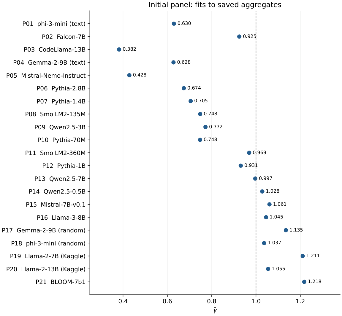
The 21 initial panel entries, using the exact estimates of Table 10. The dashed line is the mathematical infinite-support summability boundary \(\gamma =1\). It is not a measured phase transition in a network. No missing or approximate exponent is replaced by zero.
8.3 Finite-Family Quantities from the Fitted Exponents
For each full-precision fitted exponent we calculate the discrete normalizer and moments on \(d=1,\ldots ,2000\). Thus \(T_{\rm attn}=1/\widehat\gamma \), \(U=\mathbb E\log d\), \(S=\log Z_N+\widehat\gamma U\), \(I=\operatorname {Var}(\log d)\) and \(C_V=\widehat\gamma ^2I\). Extending a regression tail to this support is an additional distributional assumption. These values are neither direct attention entropies nor new measurements. In particular, the correlation of \(S\) with its input exponent does not independently validate the model. The coordinate \(\chi =1/|\widehat\gamma -1|\) is included to retain the proposed diagnostic, but it is not the finite-family Fisher susceptibility: \(I\) stays finite at one.
|
ID |
\(T_{\rm attn}\) |
\(U\) |
\(S\) |
\(C_V\) |
\(I\) |
\(\chi \) |
|
P01 |
1.5884 |
5.3149 |
7.1060 |
1.4730 |
3.7163 |
2.6995 |
|
P02 |
1.0814 |
3.9348 |
6.0208 |
4.6217 |
5.4052 |
13.2775 |
|
P03 |
2.6157 |
6.0337 |
7.4775 |
0.3204 |
2.1922 |
1.6189 |
|
P04 |
1.5933 |
5.3220 |
7.1105 |
1.4586 |
3.7027 |
2.6856 |
|
P05 |
2.3340 |
5.9271 |
7.4343 |
0.4461 |
2.4302 |
1.7496 |
|
P06 |
1.4833 |
5.1421 |
6.9933 |
1.8335 |
4.0342 |
3.0690 |
|
P07 |
1.4183 |
5.0140 |
6.9050 |
2.1142 |
4.2528 |
3.3907 |
|
P08 |
1.3369 |
4.8251 |
6.7677 |
2.5437 |
4.5465 |
3.9682 |
|
P09 |
1.2953 |
4.7139 |
6.6832 |
2.8027 |
4.7023 |
4.3866 |
|
P10 |
1.3376 |
4.8269 |
6.7690 |
2.5396 |
4.5439 |
3.9620 |
|
P11 |
1.0318 |
3.6925 |
5.7914 |
5.1444 |
5.4768 |
32.4387 |
|
P12 |
1.0740 |
3.9000 |
5.9886 |
4.6989 |
5.4199 |
14.5154 |
|
P13 |
1.0033 |
3.5416 |
5.6430 |
5.4488 |
5.4850 |
302.6061 |
|
P14 |
0.9724 |
3.3681 |
5.4674 |
5.7740 |
5.4598 |
35.2435 |
|
P15 |
0.9427 |
3.1923 |
5.2837 |
6.0720 |
5.3964 |
16.4608 |
|
P16 |
0.9565 |
3.2750 |
5.3708 |
5.9361 |
5.4310 |
21.9895 |
|
P17 |
0.8812 |
2.8018 |
4.8552 |
6.5951 |
5.1213 |
7.4186 |
|
P18 |
0.9647 |
3.3232 |
5.4211 |
5.8533 |
5.4472 |
27.3206 |
|
P19 |
0.8259 |
2.4284 |
4.4175 |
6.8753 |
4.6900 |
4.7447 |
|
P20 |
0.9483 |
3.2259 |
5.3193 |
6.0178 |
5.4115 |
18.3384 |
|
P21 |
0.8211 |
2.3954 |
4.3775 |
6.8881 |
4.6444 |
4.5909 |
Colour: blue shade = the number’s size within its column.
8.4 Observations and Mechanistic Hypotheses
C1: the finite maximum of \(C_V\).
At \(N=2000\), numerical maximization of the exact discrete sum gives \(\gamma \simeq 1.256885\) and \(C_V\simeq 6.919812\). At one, \(C_V=5.484118\), whereas the continuous approximation gives \(4.814477\). This is a property of the chosen statistical family. It neither locates an empirical network transition nor follows by treating the continuous formula as a discrete identity.
C2: large nominal bases do not determine the fitted exponent.
The initial Qwen text fits are \(1.028374\) (0.5B), \(0.772033\) (3B) and \(0.996695\) (7B). This non-monotonic sequence is not explained by a candidate depending only on shared \(\theta \) and evaluation length. For \(T=2000\) and \(\theta =10^6\), the stated Padé expression gives approximately \(0.997\). The initial Llama-3 text fit is \(1.045476\). These comparisons are tests of a proposed predictor, not confirmations from the configuration alone.
Substituting \(\widehat\gamma =.772033\) into the proposed inverse gives
This is a coordinate of the Padé model, not a recovered physical RoPE base. The Qwen-3B random fit is about \(.964\), so its corpus contrast is about \(+.192\). That observation does not prove intact geometry, absent induction heads, or a mechanism caused by two shared KV heads. Such alternatives require controlled activation or weight interventions. Likewise, large \(\theta \) alone does not count active rotary planes: the actual rotary dimension and phase threshold enter the integer count.
GQA and the proposed pressure analogy.
The ratio of query to KV heads may motivate an architectural hypothesis about shared representations. The present corpus contrast does not identify a pressure, confinement law or training threshold. A matched GQA intervention, with fixed data, distance support and loading precision, would be needed to test that hypothesis.
C3: corpus contrast is descriptive.
Define \(\Delta \gamma =\widehat\gamma _{\rm random}-\widehat\gamma _{\rm text}\). Positive, negative and near-zero contrasts all occur. Six representative pairs appear in Figure 8; the evidence manifest contains 34 available pairs. Each displayed pair is refitted on the intersection of its saved fitting grids. Matching distances does not establish identical tokenizers, prompts, seeds, precision or acquisition runs. A positive sign is not a sufficient detector of sliding-window attention, and a negative sign is not a sufficient detector of GQA or induction heads. No accuracy estimate for such a classifier is established here.
🖼️ Figure 8
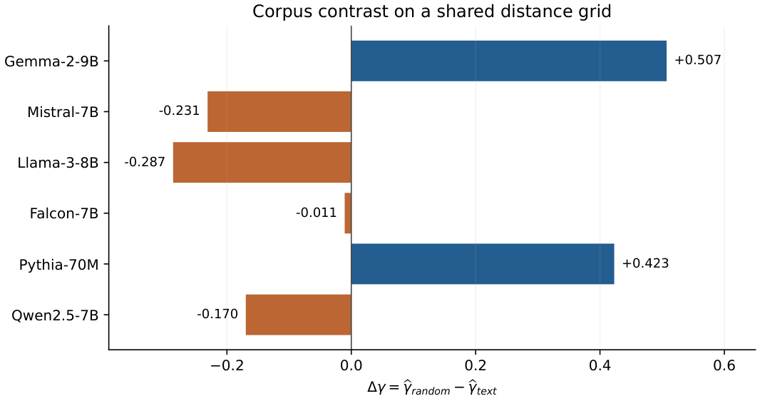
Six corpus contrasts recomputed from saved means on a common within-pair grid. Falcon uses 30–1000; the other five pairs use 30–2000. The two formerly absent random-corpus points have saved data: Pythia-70M gives \(+0.422912\) and Qwen2.5-7B gives \(-0.169680\). The bars are point estimates, without an inferred mechanism or an uncomputed confidence interval.
C4: quantization and acquisition checks.
The initial Llama-2 text record contains \(\widehat\gamma =.287057\). Comparing that number with a different platform record cannot isolate a 4-bit effect: corpus, fitting range, implementation and precision must be matched, and the Kaggle metadata discussed above are incomplete. The proposed inverse also has a strict domain: \(\widehat\gamma =1\) is singular and \(\widehat\gamma {\gt}1\) yields a negative value for positive \(T\). It is not a generally valid physical-base estimator for fp16 models. A controlled precision sweep remains the appropriate experiment.
C5: ALiBi and finite-range power-law fits.
BLOOM-7b1 has a text exponent \(1.217824\) with \(R^2=.997330\); the initial random estimate is approximately \(.882\). These fits describe sampled distances, not an infinite tail. A mixture of content scores and positional biases need not have the same functional form as its bias alone. Larger-distance data and held-out comparison of competing models are required to distinguish power, exponential and mixed tails. The MaxEnt theorem identifies an optimizer under a prescribed moment constraint; it does not demonstrate that training imposes that constraint or that a power law is a universal attractor.
C6: Pythia size series on matched distance grids.
The eight Pythia sizes biderman2023pythia retain their individual observations. The following table fits both corpora on the same distances within each pair; the last row has only three distances. This restriction changes the random estimate of Pythia-2.8B from \(.551\) on its longer recorded range to \(.790851\) on 30–100, producing \(\Delta \gamma =+.116690\). Comparing \(.551\) with the three-point text estimate would mix supports.
|
Pythia |
\(\widehat\gamma _r\) |
\(R^2_r\) |
\(\widehat\gamma _t\) |
\(\Delta \gamma \) |
\(n\) |
|
14M |
1.003714 |
0.977698 |
0.685288 |
+0.318427 |
7 |
|
31M |
1.539824 |
0.964259 |
1.235001 |
+0.304823 |
7 |
|
70M |
1.170514 |
0.994076 |
0.747602 |
+0.422912 |
7 |
|
160M |
1.017145 |
0.981723 |
0.510892 |
+0.506254 |
7 |
|
410M |
0.936235 |
0.987529 |
1.021853 |
-0.085618 |
7 |
|
1B |
0.712754 |
0.956201 |
0.931108 |
-0.218354 |
7 |
|
1.4B |
0.687585 |
0.948837 |
0.705073 |
-0.017488 |
7 |
|
2.8B |
0.790851 |
0.998392 |
0.674162 |
+0.116690 |
3 |
Colour: blue shade = the number’s size within its column.
Among the seven pairs spanning 30–2000, the sign changes between 160M and 410M, but this association does not locate an induction-head formation threshold. The 2.8B common-support result also prevents a universal post-410M sign claim. Parameter count, training evolution and mechanistic head identity are different variables.
Connection to induction-head dynamics.
Induction-head research olsson2022induction motivates testing copy-specific activation patterns and their causal contribution during training. A corpus slope contrast alone cannot identify those circuits, establish a minimum parameter count for them, or equate a size-series comparison with a training-time transition. The proposed connection remains a testable mechanism hypothesis.
🖼️ Figure 9
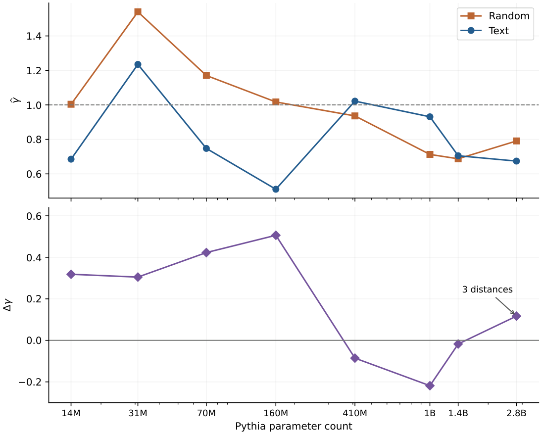
Pythia estimates and corpus contrasts on matched within-pair distance grids. The last point uses three distances, all others seven. The lines guide the eye; no induction-head labels or mechanistic threshold are inferred from the sign.
EXP-T1: training checkpoints and H3 normalization.
The saved H3 experiment contains eight checkpoints, including step 3000. It records a denominator \(\mu _{d=10}-\mu _{\rm baseline}\) and recovery statistics with 50 prompts. A negative denominator reverses the intended normalization direction; a small positive denominator is numerically unstable. These facts concern the score definition, not a Hagedorn transition. The stored \(L_{\rm crit}\) values are outputs of that protocol, not independent circuit ground truth.
|
Step |
denom |
\(L_{\rm crit,90}\) |
|
512 |
+0.3927 |
— |
|
1000 |
+0.0024 |
1 |
|
2000 |
-1.0740 |
— |
|
3000 |
-0.7385 |
— |
|
8000 |
-0.9241 |
— |
|
16000 |
-1.0837 |
— |
|
32000 |
-0.6498 |
— |
|
143000 |
+0.7085 |
4 |
Colour: grey = nothing; blue shade = the number’s size within its column.
A separate attention-profile file contains nine checkpoints and eight distances \(\{ 10,20,50,100,200,500,1000,2000\} \). Regressing the saved means reproduces its exponents. Its checkpoint set differs from H3: it includes steps 4000 and 64000, but not 3000. The table below retains that experiment separately. In particular, \(\gamma {\gt}1\) describes steeper decay within the power-law family, not maximally spread attention. Aligning the two protocols by checkpoint does not establish a causal link between their outputs.
|
Step |
\(\widehat\gamma \) |
\(R^2\) |
|
512 |
0.855025 |
0.916052 |
|
1000 |
0.856545 |
0.975162 |
|
2000 |
0.904754 |
0.988525 |
|
4000 |
0.983180 |
0.988667 |
|
8000 |
1.063573 |
0.989672 |
|
16000 |
1.001999 |
0.991789 |
|
32000 |
0.886514 |
0.991220 |
|
64000 |
0.794771 |
0.990799 |
|
143000 |
0.780527 |
0.988175 |
Colour: blue shade = the number’s size within its column.
C7: Falcon and the proposed mixed tail.
The mixed family \(A(d)=C_0d^{-\gamma }e^{-\lambda d}\) remains a useful candidate. A saved fit summary reports the following parameters, but does not include its fitting grid, loss convention or input hashes. They are retained as an unverified fit report, not as parameters reproduced by the present aggregate replay.
|
Corpus |
\(C_0\) |
\(\gamma \) |
\(\lambda \) |
\(1/\lambda \) |
\(R^2\) |
|
mongo |
0.03857 |
0.743944 |
0.00103866 |
962.780 |
0.998985 |
|
random |
0.00981 |
0.297567 |
0.00510298 |
195.964 |
0.994250 |
On the currently saved 30–1000 aggregates, the pure log-log fit gives \(R^2=.989728\) for text and \(.967807\) for random. An unconstrained log-linear mixed fit on those same points gives negative \(\lambda \) in both corpora, and therefore does not reproduce the positive-cutoff summary above. The discrepancy must be resolved from the original inputs and objective before those mixed parameters support a mechanism. Even a higher training \(R^2\) for a three-parameter model would not by itself establish induction copying, exponential dominance, or predictive superiority; comparison must account for model complexity and held-out error.
8.5 Evidence and replay protocol
The archived October atlas supplies 25 measurements among 42 historical identifiers. We recomputed the binning, regression and bootstrap from the saved NumPy profiles, and matched each row to its successful checkpoint record. The maximum exponent discrepancy was below \(3\times 10^{-15}\); the maximum interval-endpoint discrepancy was below \(1.4\times 10^{-9}\). The latter reflects storage of sequence profiles in 32-bit floats. These checks reproduce computations on saved data; they do not rerun the model or certify that its implementation was correct.
The source protocol uses text from the recorded pile-10k snapshot, selecting documents long enough for the model’s tokenizer and context, and taking their first \(T\) tokens. This does not guarantee identical documents or token sequences across models. All 25 successful records report zero non-finite attention fraction. That field is a recorded instrument check, not independently reconstructed full attention tensors. Four job records identify an immutable model revision in their own metadata; the others use mutable names or local paths. The hashes of saved profiles do not repair that limitation.
8.6 The 25 available rows
|
Model |
QL exponent [95% CI] |
T |
Precision |
|
Llama-2-7b-hf |
0.782 [0.750, 0.816] |
2048 |
bf16 |
|
CodeLlama-13b-Instruct-hf |
0.756 [0.716, 0.804] |
1024 |
bf16 |
|
Mistral-Nemo-Instruct-2407 |
0.776 [0.742, 0.811] |
1024 |
bf16 |
|
pythia-160m |
1.073 [1.047, 1.101] |
2048 |
fp32 |
|
gemma-2-9b-it |
0.842 [0.793, 0.899] |
2048 |
bf16 |
|
phi-3-mini-4k-instruct |
0.385 [0.358, 0.414] |
2048 |
bf16 |
|
pythia-2.8b |
0.867 [0.831, 0.905] |
2048 |
fp32 |
|
pythia-14m |
1.244 [1.213, 1.281] |
2048 |
fp32 |
|
pythia-1.4b |
0.930 [0.897, 0.967] |
2048 |
fp32 |
|
pythia-70m |
1.174 [1.147, 1.199] |
2048 |
fp32 |
|
gpt2-large |
0.899 [0.873, 0.924] |
1024 |
fp32 |
|
Qwen2.5-3B |
0.895 [0.841, 0.949] |
2048 |
bf16 |
|
gpt2-medium |
0.880 [0.853, 0.906] |
1024 |
fp32 |
|
OLMo-7B-hf |
0.494 [0.482, 0.506] |
1024 |
bf16 |
|
falcon-7b |
0.838 [0.811, 0.867] |
1024 |
bf16 |
|
pythia-1b |
0.974 [0.943, 1.006] |
2048 |
fp32 |
|
Qwen2.5-7B |
0.844 [0.804, 0.884] |
1024 |
bf16 |
|
gpt2-xl |
0.791 [0.766, 0.815] |
1024 |
fp32 |
|
pythia-410m |
0.984 [0.953, 1.016] |
2048 |
fp32 |
|
gpt2 |
0.873 [0.849, 0.898] |
1024 |
fp32 |
|
phi-2 |
0.782 [0.750, 0.811] |
2048 |
bf16 |
|
Meta-Llama-3-8B |
0.854 [0.811, 0.902] |
2048 |
bf16 |
|
Mistral-7B-v0.1 |
0.855 [0.815, 0.893] |
2048 |
bf16 |
|
bloom-7b1 |
1.095 [1.069, 1.127] |
1024 |
bf16 |
|
pythia-31m |
1.233 [1.203, 1.264] |
2048 |
fp32 |
Seventeen historical models have no corresponding October measurement in this reconstruction. They are missing observations, not failures with zero exponent, and are excluded from the following denominators. The table also mixes 15 contexts of 2048 and 10 of 1024, different precisions and model-specific tokenizers. Its rows should not be treated as a controlled intervention on architecture.
One model, several instruments.
Pythia-2.8B illustrates the scale of protocol dependence: E4 text gives \(0.674162\) on three distances; E4 random gives about \(0.551\) on its longer range and \(0.790851\) on the matched short support; QL at \(T=2048\) gives \(0.866809\); the field fit is about \(0.969\), its mean of cell fits about \(1.309\), and the layer-summary record about \(1.327\). These are distinct estimands and records. In particular an E4 curve samples different rows and lengths: it is not a probability vector on distances. Substituting its slope into \(p_g(d)\) constructs a new family member. Its entropy and quantiles must not be exported as measured attention mass or KV retention.
Descriptive controls in the fixed-query panel.
The eight Pythia QL point estimates decrease strictly with size: \(1.244,1.233,1.174,1.073,0.984,0.974,0.930,0.867\) (Spearman \(-1\)). At their shared nominal \(\theta =10000,T=2048\), the candidate is constant (\(0.747006\)). This is a descriptive trend in saved fits; overlapping intervals, one checkpoint per size, changing architecture and missing immutable revisions limit causal attribution to scale. GPT-2 variants, which use learned absolute positions, span about \(0.791\)–\(0.899\) and overlap the RoPE panel. A fitted distance slope therefore does not uniquely identify RoPE. These controls motivate matched prospective measurements.
Checkpoint names and identity.
The initial source JSONs identify google/gemma-2-9b-it, codellama/CodeLlama-13b-Instruct-hf and microsoft/phi-3-mini-4k-instruct; abbreviated labels such as “Gemma-2-9B” do not denote verified base checkpoints. The QL table names the same variants. Matching repository names does not establish identical weight revisions, and the separate 42-row legacy atlas must not be confused with the 21-row initial E4 panel. Historical/QL agreement remains a comparison of archived identifiers with incomplete execution provenance.
8.7 Historical agreement and the Padé comparison
The historical text exponent lies inside the October bootstrap interval for one of 25 models. Spearman correlation between historical and QL exponents is \(0.269\). The 19 rows with a stored Padé value give Spearman correlation \(-0.445\) against the QL exponent. Ties in the Padé values receive average ranks. These are descriptive calculations, not corrected significance tests or prospective predictive evaluations.
🖼️ Figure 10
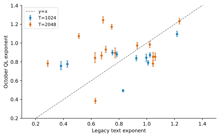
Historical text exponents against October QL fits. Error bars are the archived bootstrap intervals, reproduced from sequence profiles. The diagonal denotes equality; colors distinguish context length. Changes in corpus and protocol prevent interpreting disagreement as a causal estimate of one instrumental bias.
🖼️ Figure 11
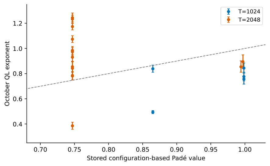
Nineteen stored configuration-based Padé values against QL fits. This analysis checks the stored comparison, not every model’s original immutable configuration. The plot does not validate Padé as a predictor.
9 Diagnostic Workflow and Instrument Controls
A fitted exponent describes the combination of an attention mechanism and a measurement protocol. The first diagnostic question is whether that protocol produces a slope on a null distribution. A high in-sample \(R^2\) cannot answer that question: the uniform control below has \(R^2=0.988452\) on the main E4 grid. The earlier speed claims and universal diagnostic thresholds are not established by this manuscript. The command examples elsewhere are historical interfaces.
9.1 Variable-length E4 has a nonzero uniform null
Groups 1–2 in Appendix K generalize this control to weighted probes and prove strict bounds and monotonicity for affine exposure.
The available E4 extractor sets the sequence length to \(n(d)=d+50\), reads the last query \(i=d+49\), and samples key \(j=49\). Thus it changes the query, available context and row normalizer with distance while holding the key index fixed. For uniform causal attention, including the query’s own key,
This is an OLS slope caused by the instrument; it does not require trained weights, positional encoding or token semantics. Its local log slope is \(d/(d+50)\), which rises with distance. The short/long slope contrast can therefore occur under a uniform null too.
|
Grid |
\(\widehat\gamma _0\) |
\(R^2\) |
|
30–2000 (7 points) |
0.782582 |
0.988452 |
|
30–1000 (6 points) |
0.741726 |
0.987211 |
|
10–2000 (8 points) |
0.681834 |
0.964115 |
|
30–100 (3 points) |
0.525737 |
0.993818 |
|
10–100 (4 points) |
0.396753 |
0.968315 |
|
200–2000 (4 points) |
0.913768 |
0.999228 |
Colour: blue shade = the number’s size within its column.
These values were checked both analytically and by passing synthetic causal attention tensors through the saved E4 extraction and fitting functions. No language model was run. For the mixture \((1-s)U_n+s\delta _0\), with constant \(s{\lt}1\) and \(U_n\) uniform on all \(n=d+50\) eligible keys, off-sink entries are \((1-s)/(d+50)\) and the slope is unchanged. If instead key zero receives exactly \(s\) and the other \(n-1\) keys share \(1-s\), entries are \((1-s)/(d+49)\): the seven-point null is \(0.785491\), rather than \(0.782582\). A context-dependent sink mass introduces another dependence. Failed heads, masks and nonfinite-value exclusions require correspondingly matched controls.
The configuration value \(\gamma _P(10^4,2000)=0.752201\) lies close to this instrumental slope, but closeness alone neither proves nor quantifies the fraction of an empirical fit caused by the confound. The former accuracy comparison cannot identify rotary geometry as the cause. Likewise, weak responses to steering or an exponent near \(0.75\) at initialization do not independently establish a learned geometric law.
9.2 Fixed queries distinguish QL from diagonal averaging
The October QL implementation uses the same query set \(Q=\{ T-\lfloor T/4\rfloor ,\ldots ,T-1\} \) at every fitted distance. Under uniform causal attention its profile is
which is constant in \(d\). In contrast, the ALL profile averages over queries \(i\ge d\) and has null
Running the actual QL accumulator and logarithmic-bin fitter on synthetic matrices gives \(|\widehat\gamma _0|{\lt}10^{-10}\) at \(T=1024\) and \(2048\), both with and without an added sink of mass \(0.2\). For ALL including key zero but without additional sink mass, the slopes are \(0.317033\) at \(T=1024\) and \(0.298064\) at \(T=2048\). The two numbers index context lengths, not the presence versus absence of a sink. These numbers use 16 bins over \([16,T/2]\); other ranges or weighting rules produce other ALL slopes. They must not be attributed to QL.
The full stored QL profile reaches \(d=3T/4\). At that last endpoint one query does sample key zero, contrary to a comment in the instrument. The fitted range \([16,T/2]\) excludes that endpoint and all key-zero terms. This boundary distinction is part of the instrument audit, not a correction to the 25 saved QL fits. A flat synthetic control verifies the reduction on that null; it does not certify real-model acquisition, masking, precision or provenance.
9.3 Report the observable and its matched control
For the same distances, exclusions and regression weights, linearity of OLS gives
The reproducibility package records this diagnostic for all 21 initial-panel rows, retaining each original slope, grid and source. It assumes the recorded row was acquired with the declared \(d+50\) procedure; incomplete provenance is not repaired by that assumption. The excess slope is not automatically a causal or learned exponent, and fitting a ratio does not turn it into a normalized probability distribution. Corpus comparisons must also use common within-pair supports.
A prospective measurement should fix context length and query positions, state whether self and sink keys are excluded, and archive per-sequence profiles, exclusions, model/tokenizer revisions, attention implementation, precision, corpus and seed. Uniform causal, uniform-plus-sink, randomized weights and shuffled-token controls answer different questions. Only the first two synthetic controls are executed in this revision. Alternative families should be compared on held-out sequences under the same observation and loss conventions. Resample sequences, not individual distances, for uncertainty when sequence-level records exist.
9.4 Derived family quantities and inverse coordinates
For a declared finite power-law family, compute \(Z_N\), entropy, Fisher information and \(C_V\) by finite sums. These quantities describe that family; they do not establish model sensitivity to context changes. \(1/\gamma \) is a formal temperature only when nonzero, and positive-temperature interpretation requires \(\gamma {\gt}0\). The intervals around \(0.95\) and \(1.05\) were heuristic labels, not validated architecture classifiers.
The correct inverse of the rational candidate at fixed \(T{\gt}0\) is
It is a positive algebraic coordinate on that domain. It does not recover a physical training base from an observed slope. The former expression \(T\sqrt2/(1-g)\) is the inverse of a linear approximation; substituting \(g=\gamma _P(\theta ,T)\) gives \(\theta +T/\sqrt2\), not \(\theta \). Exponents at or above one cannot be inverted into a positive base by the candidate.
9.5 Divergence from a declared reference
For positive normalized reference \(q\) and observed probability \(p\) on the same support, a descriptive discrepancy is
The available diagnostic script normalizes sparse sampled distances with equal point weights, rather than reconstructing all token distances or bin masses. Its KL therefore refers to that sampled support. Neither a small KL nor the old cutoff \(0.05\) identifies a positional circuit, attention sink or induction head. Circuit attribution needs functional evidence beyond a residual.
|
Historical entry |
\(\widehat\gamma \) |
KL |
|
Gemma-2-9B (random) |
1.135 |
0.075 |
|
Mistral-7B-v0.1 |
1.061 |
0.041 |
|
LLaMA-3-8B |
1.046 |
0.018 |
|
LLaMA-2-7B (reported fp16) |
1.026 |
0.002 |
|
Qwen2.5-7B |
0.997 |
0.011 |
|
Pythia-1B |
0.931 |
0.004 |
|
Pythia-70M |
0.748 |
0.008 |
|
Pythia-2.8B |
0.674 |
0.001 |
|
SmolLM2-135M (older pair summary) |
0.902 |
0.009 |
Colour: blue shade = the number’s size within its column.
The SmolLM2-135M input \(0.902\) is the rounded \(0.9019\) in the separate 21 April base/instruct summary, labelled random in the master summary. It is not the E4 text result P08 (\(0.747996\)); the available E4 random array instead replays to \(0.626655\). The older pair summary has no per-distance means for this row, so its acquisition cannot be reconstructed here. Its KL value remains a historical report. The same older exponent is retained as an explicit historical input in Table 16, solely to audit the quantile arithmetic; it is not substituted for P08.
9.6 Reassessment of the four historical cases
LLaMA-2-7B.
The reported \(0.287\) and \(1.026\) slopes are retained as historical records, but the recovered arrays and notes disagree (Section 8). They do not certify a matched fp16/4-bit effect, size invariance or an NTK recommendation. A value above one also lies outside the positive-base inverse domain.
Mistral-7B-v0.1.
The old random/text pair \(0.830/1.061\) is a protocol-specific report. The official configuration declares a 4096-token sliding window; a sequence of at most 2050 tokens does not exclude a key by that window. A direct SWA-mask mechanism therefore cannot explain this short-context contrast. The configuration source is https://huggingface.co/mistralai/Mistral-7B-v0.1/blob/main/config.json. Architectural and training differences remain possible confounds, and \(\Delta \gamma \) is not a GQA detector.
Qwen2.5-7B.
A fitted value \(0.997\) does not imply purely positional attention. The limiting continuous calculation is \(2000^{0.9}=935.248\), while using \(g=0.997\) gives a different quantile. Neither is a measured token-retention or accuracy result; the discrete values are tabulated below.
Pythia-2.8B.
Its initial text fit uses only distances 30, 50 and 100. The uniform null on that grid is \(0.525737\), and common-support comparison changes the random/text contrast. No long-context safety, stability or optimal cache policy follows from that three-point exponent.
10 Layer Heterogeneity and the Proposed Critical Layer
Layer-resolved profiles, recovery interventions and representation similarity measure different observables. Their agreement should be tested under a common protocol rather than built into the definition of a boundary. This section preserves the original layer reports while separating a proposed configuration formula from measured thresholds.
10.1 A candidate layer coordinate
For \(\theta {\gt}1\), \(T{\gt}0\), \(N_L\) layers and head dimension \(d_{\rm head}{\gt}0\), define
This is the historical configuration proposal previously denoted \(L_{\rm crit}\). Its full-head factor also ignores partial RoPE: Pythia-1B has \(d_{\rm head}=256\) but \(d_{\rm rot}=64\). Replacing one by the other would define a new candidate, not validate the old formula. Its value need not be an integer or lie in \([0,N_L]\); rounding and any clipping must be stated before comparing it to a measured layer index.
↳ Not used by another result of the paper.
En palabras.
\(L_{\rm pred}\) conserva una propuesta histórica de coordenada de capa como fórmula candidata. Usa la dimensión completa del head, aunque algunas arquitecturas rotan solo una parte.
Alcance.
No se ha validado como frontera de capa. Puede quedar fuera del intervalo de capas o no ser entero; cualquier redondeo o recorte debe declararse.
The identity \(\operatorname {sd}(\mathrm{Unif}[0,1])=1/\sqrt{12}\) does not derive the empirical architecture exponent. GPT-2 has learned absolute positions and no RoPE base to substitute in this equation. Its historical layer reports remain observations under another protocol, not evaluations of the RoPE formula.
|
Model |
\(N_L\) |
reported \(L_{\rm crit}\) |
\(\alpha \) |
old prediction |
old fit |
|
Pythia-70M |
6 |
4 |
.667 |
.748 |
.748 |
|
Pythia-1B |
16 |
15 |
.938 |
.931 |
.931 |
|
GPT2-medium |
24 |
23 |
.958 |
— |
— |
|
GPT2-large |
36 |
35 |
.972 |
— |
— |
Colour: grey = nothing; blue shade = the number’s size within its column.
10.2 A mixture does not have the average exponent
Group 3 in Appendix K proves the local-slope, curvature and global-regression statements for any finite positive mixture of powers.
For positive coefficients and two component profiles, the exact local slope is
The weights depend on distance unless the component exponents coincide or one component vanishes. A global OLS slope of an averaged attention profile therefore need not equal a layer-fraction-weighted mean of fitted exponents. That equality also fails to account for finite normalizers and failed fits.
The list \(1.35,1.41,1.12,1.10\) for Pythia-70M survives as a rounded manuscript report; its original layer-profile record was not recovered. It must not be identified with the per-head matrix used for P3 in Section 5.6. That matrix gives finite-head layer means \(1.918196,1.663184,1.529207,1.082143\) for L0–L3, with L4–L5 missing; the L1–L3 mean is \(1.424844\), whereas the old list gives \(1.210000\) there. For the old four-entry list, the arithmetic mean is \(1.245\); multiplying by \(4/6\) gives \(0.830\), not \(0.748\). Even the corrected arithmetic is not a derivation of the global slope. The entries marked NaN in layers 4–5 denote unavailable or rejected fits, not an exponent zero or proof of semantic processing. The duplicate reported and predicted values in the old table are not independent validation without the original fitting and parameter-selection record.
10.3 CKA is a separate observation
The companion analysis marin2026coordination was cited for adjacent-layer CKA values near one before a proposed boundary and below \(0.5\) afterwards. Those historical claims are preserved in the audit record. A CKA change can motivate a shared analysis, but does not by itself identify positional versus semantic computation or validate Equation (50). A confirming test must specify the same checkpoint, examples, representations, indexing and threshold selection, and evaluate agreement on held-out observations.
10.4 Training checkpoints and recovery normalization
The saved H3 experiment has eight checkpoints, including step 3000, and uses 50 prompts. Its recovery normalization contains \(\mu _{d=10}-\mu _{\rm baseline}\). A negative denominator reverses the intended direction; one close to zero amplifies numerical variation. A missing or unstable threshold does not imply that a physical layer boundary ceases to exist. The stored threshold outputs and denominators are preserved in Section 8 and in the reproducibility package.
The attention trajectory has nine checkpoints, including 4000 and 64000 but not 3000. These are separate protocols. Its fitted exponent exceeds one at steps 8000 and 16000, not throughout steps 2000–32000. Within the power-law family, a larger positive exponent means steeper decay, not maximally spread attention. Agreement at the final checkpoint does not establish a stable attractor, a formation time for induction heads or an evaporation mechanism. Those interpretations need independent circuit interventions.
11 KV-Cache Compression: Mass Budgets and Recorded Tests
Groups 4 and 6 in Appendix K prove the discrete quantile order and the exact frozen-row truncation identities, including their domains and sharp bounds.
A mass quantile answers a distributional question on a declared support. It does not by itself identify a quality-preserving cache policy. In particular, the variable-length E4 fits have the instrumental confound demonstrated in Section 9.1. The family calculations below remain mathematically valid, while using a fitted model slope as their input requires a matched measurement and evaluation protocol.
11.1 Continuous and discrete windows
For density proportional to \(d^{-g}\) on \([1,N]\), \(N{\gt}1\), and \(0{\lt}f{\lt}1\), the unique \(f\)-mass quantile is
For token distances \(\{ 1,\ldots ,N\} \) with counting measure, the corresponding exact quantile is instead \(D_{f,N}=\min \{ k:\sum _{d=1}^k d^{-g}\ge f\sum _{d=1}^N d^{-g}\} \). For the discrete case \(N\) is an integer. Both quantiles are defined for every finite real \(g\); they do not include a self key at \(d=0\) or a separately modelled attention sink.
↳ Not used by another result of the paper.
For \(g\ne 1\), dividing \(\int _1^D d^{-g}\, \mathrm{d}d\) by \(\int _1^N d^{-g}\, \mathrm{d}d\) gives \((D^{1-g}-1)/(N^{1-g}-1)\); both integrals contain the factor \(1/(1-g)\). Equating this ratio to \(f\) yields the stated formula. At \(g=1\), the ratio is \(\log D/\log N\). In either case the cumulative density is strictly increasing. On the discrete support, partial sums increase strictly and the smallest index meeting the mass condition is unique.
En palabras.
En la densidad continua proporcional a \(d^{-g}\) sobre \([1,N]\), integrar y resolver la masa acumulada da un cuantil explícito, con el caso \(g=1\) igual a \(N^f\). Para distancias enteras, el cuantil exacto es el primer índice cuya suma parcial alcanza la fracción pedida. Los dos cuantiles no son intercambiables y ninguno garantiza precisión en una tarea KV.
Alcance formal.
La prueba analítica figura en el paper; la ficha no atribuye una prueba Isabelle de toda la fórmula continua ni de rendimiento del modelo.
🧪 Lab: Figure 12 live: continuous and integer mass windows
Recompute both quantiles of the finite power family; the integer one is a partial-sum threshold.
For fixed \(g{\lt}1\) and \(f\), the large-\(N\) approximation is \(D_{f,c}\sim Nf^{1/(1-g)}\). It is not uniform as \(g\to 1\) at fixed \(N\). For fixed \(g{\gt}1\) the continuous quantile tends to \((1-f)^{-1/(g-1)}\) as \(N\to \infty \); this is not a geometric-series argument and its accuracy at a particular finite \(N\) must be checked.
🖼️ Figure 12
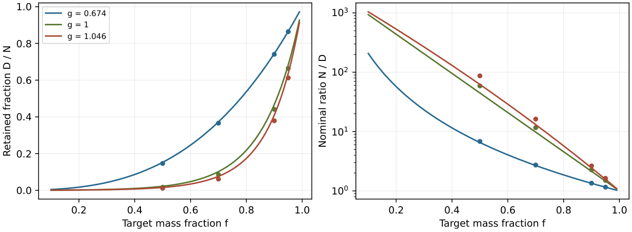
Family calculations on \(N=2000\): continuous quantiles (lines) and discrete token-distance quantiles (markers). The inputs are illustrative exponents, not calibrated model policies. The continuous quantile is smooth through \(g=1\); the discrete quantile is integer-valued and can have steps. Neither has a special task-accuracy threshold there.
|
Historical input |
\(g\) |
\(D_{.9,c}\) |
\(D_{.9,N}\) |
\(D_{.5,c}\) |
\(D_{.5,N}\) |
|
LLaMA-2-7B |
1.026 |
870.9 |
813 |
37.1 |
27 |
|
Pythia-2.8B |
0.674 |
1489.5 |
1482 |
305.5 |
293 |
|
Pythia-70M |
0.748 |
1404.2 |
1392 |
220.4 |
205 |
|
SmolLM2-135M (older input) |
0.902 |
1153.3 |
1121 |
89.3 |
74 |
|
Pythia-1B |
0.931 |
1093.4 |
1056 |
73.2 |
59 |
|
Qwen2.5-7B |
0.997 |
942.5 |
891 |
45.7 |
34 |
|
LLaMA-3-8B |
1.046 |
820.2 |
758 |
32.1 |
23 |
Colour: blue shade = the number’s size within its column.
The table retains the original rounded exponent inputs so that the arithmetic change can be isolated. Its model names identify those historical inputs, not validated present-day measurements. For example, at \(g=0.674\) the half-mass window is about 305.477 continuously and 293 discretely; the previous 987 was not the quantile of this family. At \(g=0.75\), \(N=2000\) and \(f=0.9\), the corrected schematic values are \(1401.606\) (continuous) and \(1389\) (discrete).
The actual empirical mass should be measured on a fixed, appropriate support, rather than substituted by either calculation without testing the fit.
11.2 A conditional output bound and actual cache allocation
Let a frozen attention row have weights \(p_j\), values \(v_j\) and removed mass \(0\le \epsilon {\lt}1\). After removing those entries and renormalizing the retained weights, write the retained and removed conditional means as \(o_K,o_R\). For \(\epsilon {\gt}0\), \(o=(1-\epsilon )o_K+\epsilon o_R\), hence
The zero-mass case is immediate. The first inequality follows because both conditional means are convex combinations of the values. A subsequent linear projection adds its induced operator norm. This is a frozen-row bound; it does not cover altered hidden states, repeated autoregressive steps or task accuracy after eviction.
For a conventional unexpanded dense cache with \(L\) layers, \(H_{\rm KV}\) key/value heads, head dimension \(d_{\rm head}\) and \(b\) bytes per scalar, physically evicting \(N-W\) tokens saves \(2bLH_{\rm KV}d_{\rm head}(N-W)\) bytes per sequence, before allocator overheads. GQA uses the KV-head count, not the query-head count. Biasing scores or setting weights to zero does not itself reduce a dense allocation. For the old illustrative input \(g=1.046\), \(N=8192\), \(f=0.9\), the continuous window is \(2757.511\), a nominal \(66.34\% \) reduction; the discrete window is \(2537\), a \(69.03\% \) reduction.
These are mass-budget calculations; they neither establish the attention profile at length 8192 nor certify a longer usable context.
11.3 EXP-B2: the windows actually evaluated
The saved two-model record specifies \(N_{\rm full}=2048\), 120 samples and 64 evaluated targets per sample on WikiText-2 test. The available code uses \(W=\operatorname {round}(Nf^{1/(1-g)})\), with a minimum of 64 and a full-window fallback for \(g\ge 1\). Thus the trials at \(W=445\) and \(1482\) test that asymptotic rule, not the exact finite quantile in the theorem.
|
Model |
\(g\) |
tested \(W\) |
full PPL |
\(\Delta \)PPL(\(W\)) |
\(\Delta \)PPL(1024) |
|
pythia-1b |
0.931 |
445 |
11.7956 |
+1.4443 |
-0.1433 |
|
pythia-2.8b |
0.674 |
1482 |
9.2421 |
-0.5141 |
-0.0126 |
For the same rounded inputs and \(N=2048\), the exact 90% windows are \(1117.959\) continuously and \(1079\) discretely for Pythia-1B, and \(1524.892\) and \(1518\) for Pythia-2.8B. These are newly recalculated family quantities, not windows that were evaluated in the saved trials. The numerical coincidence between 1482 and a discrete quantile at \(N=2000\) does not change the experiment’s recorded \(N=2048\).
The script samples each target start from an interval whose lower endpoint is \(W\). Reusing seed 42 therefore does not keep target positions identical between windows. Moreover, during the 64 teacher-forced predictions the available prefix grows from \(W\) to \(W+63\); this is not a rolling cache-eviction benchmark with fixed context at every target. Saved aggregates alone cannot recover paired confidence intervals or distinguish a window effect from changes in sampled positions. Negative sample \(\Delta \mathrm{PPL}\) does not prove that the discarded tokens were noise.
Separate seven-model extension.
The extended record retains seven models and uses the same asymptotic rule. Its available script specifies 120 samples and 32 targets per sample, whereas the JSON omits those two settings. This evidence supports a source-code description, not a certificate of the exact historical runtime.
|
Model |
\(g\) |
tested \(W\) |
\(W/N\) |
\(\Delta \)PPL |
stored knee |
|
pythia-14m |
0.685 |
1466 |
71.6% |
+4.3765 |
1280 |
|
pythia-70m |
0.748 |
1348 |
65.8% |
-1.1329 |
1024 |
|
pythia-160m |
0.511 |
1651 |
80.6% |
+1.4443 |
1024 |
|
pythia-410m |
1.022 |
2048 |
100.0% |
+0.0000 |
768 |
|
pythia-1b |
0.931 |
445 |
21.7% |
+0.9997 |
768 |
|
pythia-1.4b |
0.705 |
1433 |
70.0% |
-0.1715 |
768 |
|
pythia-2.8b |
0.674 |
1482 |
72.4% |
-0.3408 |
768 |
Colour: blue shade = the number’s size within its column.
The two displayed \(+1.4443\) entries are a rounding coincidence: the original Pythia-1B JSON gives \(13.2399089962-11.7955767485=1.4443322477\), while the extended Pythia-160M JSON gives \(23.9412332628-22.4969311427=1.4443021201\). They are distinct saved differences, both reproduced from their recorded PPLs.
The different Pythia-1B and 2.8B deltas in the two panels belong to separate runs and must not be merged. Pythia-14M has \(g=0.685\) yet positive \(\Delta \mathrm{PPL}\) in the extended panel, so the observations do not establish a universal favorable interval such as \([0.65,0.85]\). The 410M entry uses the full window and is not a successful compression trial. The recorded heuristic knee depends on the sampled sweep and its criterion; no optimum or general replacement \(f=0.93\)–\(0.95\) follows from this record.
11.4 Power-law attention allocation: conditional mass budgets
For the discrete family with \(\gamma {\gt}0\), weights decrease with distance. Among sets of a fixed cardinality \(D\), the first \(D\) distances maximise retained family mass. Their mass is
The minimum integer budget attaining mass at least \(f\) is the discrete quantile \(D_{f,N}\) of Theorem 11.1. This result concerns the ideal family, not content-dependent token rankings, task accuracy or an optimal sparse kernel. At \(\gamma =0\) all sets of that cardinality tie; at negative \(\gamma \) the largest family weights are at the greatest distances. A recent-window interpretation therefore requires the positive-exponent condition.
Continuous approximation and threshold algebra.
For fixed \(0{\lt}\gamma {\lt}1\) and \(0{\lt}f{\lt}1\), the continuous quantile satisfies
The second expression is the average retained density, not its boundary threshold. The continuous density at the boundary instead satisfies \(p_c(D_{f,c})\sim (1-\gamma )f^{-\gamma /(1-\gamma )}/L\). An inverse-length dependence in an empirical method such as BLASST blasst2025 does not identify its calibrated coefficient with either expression. The former exponent \(f^{1/(1-\gamma )}\) in the average-density calculation was an algebraic error. Configuration lookup cannot replace the method’s calibration on the basis of this calculation.
Comparison with PyramidKV.
PyramidKV cai2024pyramidkv reports experiments retaining \(12\% \) of the KV cache. Its layer-dependent selection is different from retaining a fixed distance window. To examine the numerical comparison previously made here, take \(\gamma =1.05\) as an illustrative family input, not a Padé prediction: the latter is always below one for positive inputs. At \(N=8192\), the exact continuous formula gives
These replace the former \(0.27\), \(0.13\) and asserted \(12\% \) association with \(f=0.78\). Token-distance quantiles use finite sums instead. Neither numerical agreement nor choosing \(f\) after seeing an external budget predicts the external method’s accuracy.
Reasoning and long-context performance.
SnapKV, PyramidKV, H2O and reasoning-focused compression studies snapkv2024,cai2024pyramidkv,zhang2023h2o,holdontothat2025,blasst2025 provide task-specific empirical comparisons. They do not establish that a mass quantile preserves reasoning. The earlier reported benchmark values are preserved in the separate predecessor archive indexed by Appendix J; they were not rerun for this revision. Likewise, \(1/\gamma \) is a threshold-count exponent under the stated family, not a demonstrated geometric dimension that forbids multi-hop reasoning when \(\gamma {\gt}1\). Test quality, retained positions, attention sinks, memory and latency directly for each proposed intervention.
11.5 Shifted-base ratio: scope of the former information-loss expression
Define the algebraic shifted-base coordinate \(b(x)=\theta +x/\sqrt2\). The quantity formerly denoted an information loss is the signed log ratio
It vanishes at \(D=N\) and its algebraic extension to \(D\to 0\) tends to \(\log \theta -\log (\theta +N/\sqrt2)\). This is a difference of logarithms, not the previously printed ratio of logarithms. The expression is nonpositive; it is not established as Shannon entropy loss, KL divergence or task error. The endpoint \(D=0\) is an extension of this coordinate, not a quantile of the continuous support \([1,N]\). Within the coordinate definition the formula is exact and requires no first-order error estimate.
11.6 Soft Horizon Decay: a tested score-bias proposal
The proposed distance weight can be studied as a chosen intervention, without interpreting its cutoff as a physical horizon. For \(h{\gt}0\), \(g{\gt}0\) and causal distance \(d\ge 0\), define
Adding \(\log w(d)\) to pre-softmax scores produces weights proportional to \(w(d)e^{s_{ij}}\), with zero weights represented by a mask. This changes their normalization and mass budget; it is not equivalent to scaling both K and V. Smooth decay of \(w\) does not establish an aliasing mechanism or superior predictions. The available implementation rounds the inverse-coordinate cutoff to an integer and uses a dense four-dimensional mask with eager attention. Its memory consumption is not a measured KV-cache saving.
The archived test used three Pythia models, length 4096, 30 chunks, WikiText-2 test and bf16 in the available script. Pythia’s training context is 2048 tokens, so this is a \(2\times \) extrapolation setting. The elevated full-attention baseline and the improvements under some masks can reflect mitigation of extrapolation failure; they do not establish in-context KV compression. An otherwise matched test at 2048, actual eviction, memory and latency measurements are needed for that claim. The cutoffs for both 1.4B (\(h=2447\)) and 2.8B (\(h=2754\)) exceed 2048; cutoff position alone does not explain their different signs. All four recorded policies are retained below. The column labelled hard \(D_f\) records the window selected by that script, not an empirical quantile of the actual attention matrix.
|
Model |
\(g\) |
\(h\) |
baseline |
hard cutoff |
soft |
hard \(D_f\) |
|
pythia-2.8b |
0.674 |
2754 |
113.533 |
120.232 |
118.843 |
120.910 |
|
pythia-1.4b |
0.705 |
2447 |
53.657 |
31.655 |
25.161 |
48.386 |
|
pythia-1b |
0.931 |
505 |
79.087 |
25.261 |
26.721 |
19.955 |
Colour: blue shade = the number’s size within its column.
For Pythia-2.8B, soft decay reduces PPL by \(1.155\% \) relative to hard cutoff but raises it by \(4.678\% \) relative to the full-attention baseline. The old “21%” can be recovered only as a \(20.729\% \) reduction of the excess PPL above that baseline, a different denominator. Pythia-1.4B has a \(20.514\% \) relative PPL reduction against hard cutoff. Pythia-1B favors the tested hard \(D_f\) policy. The lowest recorded PPL among all four policies is therefore baseline for 2.8B, soft decay for 1.4B and hard \(D_f\) for 1B.
The available script resets the sampling seed per policy, which requests the same chunk starts for a fixed tokenized corpus. It does not store per-chunk losses or actual finite-example counts, and skips nonfinite losses. Its aggregate standard deviations are not paired confidence intervals. The rule \(h\gtrsim T_{\rm train}/2\) was inferred from three cases, not validated as an operating boundary. Hard truncation specifically at \(T_{\rm train}\) was not one of these four policy columns. Neither it nor the explanation that all policies retain equal attention mass is justified by this test.
11.7 Coordinate pruning and the rotary-subspace audit
The original hypothesis proposed that high-index frequency components become redundant beyond \(L_{\rm crit}\). Its prerequisites are unestablished: a failed power-law fit does not identify a semantic layer, and the Shannon entropy bound does not prescribe a sufficient set of positional coordinates. The saved ablations are retained as coordinate interventions with the limitations below.
What the available script changes.
For the fused NeoX projection reshaped as \(W[h,t,r,c]\), with \(t\in \{ Q,K,V\} \), output coordinate \(r\) and input coordinate \(c\), the archived operation is
These are output rows in the stored linear-weight convention, not input columns. The code calculates \(k_0\) from full head dimension and a \(\pi \) threshold, without consulting the partial rotary dimension or pairing.
|
Pythia |
Q heads |
\(d_{\rm head}\) |
rotary dims |
rotary pairs |
cycled pairs |
|
70m |
8 |
64 |
16 |
8 |
6 |
|
1b |
8 |
256 |
64 |
32 |
21 |
|
1.4b |
16 |
128 |
32 |
16 |
11 |
|
2.8b |
32 |
80 |
20 |
10 |
7 |
Colour: blue shade = the number’s size within its column.
The four frozen Pythia configurations set rotary_pct=0.25. In the inspected NeoX implementation, rotation acts on the first \(r=d_{\rm head}/4\) Q/K coordinates, paired as \((k,k+r/2)\); the remainder bypass rotation. For the recorded 1B threshold \(k_0=91\), the script masks coordinates 182–255, entirely outside the 64-dimensional rotary subspace. For 2.8B, \(k_0=29\) masks 58–79, outside the 20-dimensional subspace. Thus these masks cannot be called removal of uncycled RoPE planes under the audited configurations. The exact installed code and configuration of the historical run are not recorded; the current source/config audit identifies the inconsistency without reconstructing those executions.
The corresponding theoretical fraction of Q/K weight entries set to zero is \((N_L-L_{\rm prune})/N_L\, (d_{\rm head}/2-k_0)/(d_{\rm head}/2)\). With five of 16 layers and \(37/128\) selected coordinate pairs, it is \(9.033\% \), not \(14.5\% \). Zeroing entries of an unchanged dense matrix does not itself deliver a measured memory, latency or arithmetic saving.
|
v2 model |
\(L_{\rm prune}\) |
Q/K % |
PPL |
\(\Delta \)PPL |
accuracy |
\(\Delta \)acc. |
|
pythia-1b base |
— |
0.000 |
14.9736 |
0 |
0.570 |
0 |
|
pythia-1b |
11 |
9.033 |
16.5365 |
+1.5629 |
0.405 |
-0.165 |
|
pythia-1b |
13 |
5.420 |
15.5490 |
+0.5753 |
0.550 |
-0.020 |
|
pythia-1b |
15 |
1.807 |
15.1637 |
+0.1901 |
0.540 |
-0.030 |
|
pythia-1b |
16 |
0.000 |
14.9736 |
+0.0000 |
0.570 |
+0.000 |
|
pythia-2.8b base |
— |
0.000 |
11.4973 |
0 |
0.615 |
0 |
|
pythia-2.8b |
17 |
12.891 |
14.0789 |
+2.5816 |
0.425 |
-0.190 |
|
pythia-2.8b |
19 |
11.172 |
13.2943 |
+1.7969 |
0.485 |
-0.130 |
|
pythia-2.8b |
21 |
9.453 |
12.8873 |
+1.3899 |
0.475 |
-0.140 |
|
pythia-2.8b |
23 |
7.734 |
12.4181 |
+0.9207 |
0.530 |
-0.085 |
Colour: grey = nothing; blue shade = the number’s size within its column.
The v1 Pythia-1B record retains the rows at 13, 15 and no-op cutoffs at 16, 17 and 19. Its repeated baseline rows are not independent replications. The v2 records contain the full sweeps shown above, plus their recorded baseline losses. Both available v2 scripts request 100 chunks of 1024 tokens and 200 LAMBADA examples. The latter metric is all target subtokens correct under teacher-forced argmax, not a newly run generation benchmark.
|
Selected data |
\(n\) |
OLS slope |
intercept |
\(r\) |
origin slope |
|
1B v1, positive points |
2 |
0.106627 |
-0.002562 |
1.000000 |
0.106060 |
|
1b v2, positive points |
3 |
0.189964 |
-0.253495 |
0.969389 |
0.153883 |
|
1B v2, including no-op |
4 |
0.168560 |
-0.103117 |
0.969777 |
0.153883 |
|
2.8b v2, positive points |
4 |
0.313581 |
-1.561517 |
0.988316 |
0.167242 |
Colour: blue shade = the number’s size within its column.
All fits in this table use the stored unrounded values and percent of Q/K entries as the predictor. Changing which sweep or no-op baseline rows are included changes the slope. Neither \(r{\gt}0.99\) for both models nor a common \(0.175\pm 0.005\) coefficient is reproduced. The reported interval was not a confidence interval. The positive-cost observations disfavor the original cost-free layer-cutoff proposal; they do not establish a universal linear law or a privileged set of geometric frequency components.
Relation to frequency-aware methods.
FASA fasa2026 is a separate empirical approach. These ablations do not demonstrate equivalence to its frequency chunks, establish that only uncycled planes should be retained or provide a calibration-free replacement. A follow-up must first inspect the actual rotary subspace and tensor pairing, then use matched masks, equal intervention budgets and task-level evaluation. The proposal and all earlier numerical claims remain in the archived source; no novelty or deployment prescription is inferred from this revision.
12 Context Extension: Inverse-Candidate Algebra and Empirical Tests
The configuration-based Padé candidate can be inverted exactly. Its inverse does not establish an optimum for neural-tangent-kernel scaling, retrieval or perplexity. For a specified candidate target \(-1{\lt}g{\lt}1\) and \(T{\gt}0\), define
The old notation \(\alpha _{\rm opt}\) is ambiguous: some historical tables use this candidate ratio, whereas the B1 scripts clip a different exponential expression at 64. Neither notation establishes a task optimum. The exponential expression \(e^{C/g}/\theta _{\rm nominal}\) and the linear inverse \(T\sqrt2/(1-g)\) are different functions; neither may replace Equation (56).
For \(T=2048\) and \(\theta _{\rm nominal}=10{,}000\), a target \(g=0.5\) gives \(\theta _{\rm design}=4344.464\) and \(\alpha _{\rm cand}=0.434446\). A target \(g=0.85\) gives \(\theta _{\rm design}=17860.574\) and \(\alpha _{\rm cand}=1.786057\). These correct the rounded arithmetic previously printed as 4346 and 17,858. The nominal candidate is about \(0.7470\); lowering it to \(0.5\) broadens the ideal positive power-law family. It does not establish that the corresponding trained model becomes more global or more local.
Relation to context-extension methods.
In the NTK-aware convention described by peng2023yarn, a context parameter \(s\) changes the base by \(s^{d_r/(d_r-2)}\), for rotary dimension \(d_r{\gt}2\). Thus a base multiplier \(\alpha \) corresponds algebraically to \(s=\alpha ^{(d_r-2)/d_r}\) in that convention; it is not \(s\) itself. YaRN combines a frequency-dependent schedule with attention rescaling and has its own empirical evaluations. A ratio of RoPE bases is not automatically the scaling parameter of those methods. Neither matching a reported scale nor changing a configuration field alone demonstrates the correct runtime rotary transformation. Model-specific implementations and their caches must be checked in any new experiment.
12.1 Designing a candidate base for a specified exponent
Solving the rational equation gives
Its domain is \(-1{\lt}g{\lt}1\), with the positive-exponent subfamily \(0{\lt}g{\lt}1\) used in the illustrative table. The limit as \(g\to 1^-\) is infinite for this candidate. This is not a theorem that trained models cannot have exponent one at a finite base. Task names previously attached to these targets are removed because the numerical formula does not validate those task assignments.
|
\(g\) |
\(\theta _{\rm design}\) at \(T=4096\) |
\(\theta _{\rm design}\) at \(T=8192\) |
|
0.50 |
8,689 |
17,378 |
|
0.65 |
13,654 |
27,308 |
|
0.75 |
20,274 |
40,548 |
|
0.85 |
35,721 |
71,442 |
|
0.95 |
112,956 |
225,912 |
Colour: blue shade = the number’s size within its column.
For reference, \(\theta =10{,}000\) at \(T=4096\) gives \(\gamma _P=0.550831\), not \(0.75\). The same candidate at \(T=8192\) gives approximately \(0.2664\). All table cells are generated from the equation before rounding; the archived table records the displaced values.
Testing a candidate setting.
Specify the task and target context before choosing settings. Establish a baseline, implement and verify the actual rotary transformation, and measure both profile changes and task quality under matched data and precision. The previous suggested thresholds \(g\le 0.85\) and \(\alpha \le 8\) are not universal stability constraints. The retained retrieval experiments, including their short-context degradation at a larger tested scale, apply to the conditions reported in Section 18 and Figure 17. The full previous workflow and callback remain in the separate predecessor archive indexed by Appendix J.
Relation to compression.
A candidate target is not a measured exponent. Compute a mass window from a measured profile on the intended support, or explicitly label it a hypothetical family calculation. Task validation remains necessary even if the fitted exponent agrees with the candidate target.
12.2 The former information horizon as an inverse coordinate
The function previously called an information horizon is
It is the inverse of the candidate with respect to context length. In particular, \(d_{\rm inv}(\theta ,\gamma _P(\theta ,T))=T\) and \(d_{\rm inv}(\theta _{\rm design}(g,T),g)=T\). These equalities are algebraic identities, not independent predictions of training context or retrieval failure. At a fixed \(g\), \(d_{\rm inv}(\alpha \theta ,g)=\alpha d_{\rm inv}(\theta ,g)\), but an intervention need not preserve the fitted exponent. For \(g{\gt}1\) this expression is negative and does not define a physical context length.
The previous example \(\theta =10{,}000\), \(\widehat\gamma =0.748\) gives about 2039 tokens. Its proximity to the 2048-token training context does not establish a universal ceiling. EXP-B1v4 records \(88\% \) at nominal length 3072 and \(10\% \) at 4096 without base scaling; the assertion that it validates \(L^c=2d_{\rm inv}\) is withdrawn. A uniform needle’s expected distance \(L/2\) alone cannot determine a retrieval curve or a collapse threshold. No general impossibility claim for fine-tuning, decoding or prompt changes follows.
For \(z=T\sqrt2/\theta {\gt}0\), the same algebra yields
The constant depends on the stated definition of \(z\). It is an identity of coordinates, not an empirical invariant of a model.
12.3 Future direction: testing a feedback controller
The original thermostat increased \(\theta \) when a measured exponent exceeded an illustrative target. That direction conflicts with the positive derivative of the candidate in Section 3. A purely candidate-based sign correction would instead use the unvalidated rule
This displayed rule records the direction implied by the candidate only; it is not a recommended implementation. Correcting that sign does not establish the response of a trained network, stability, reduced loss spikes or preserved retrieval. The proposed constants \(g_*=0.85\), \(\delta =0.05\) and \(\eta =0.1\) were illustrative choices without a validated universal operating range.
A useful controlled study would measure the response to small base changes, estimate uncertainty and lag, then compare a prespecified controller with fixed-base and matched-compute baselines. Report instability, loss, task scores and overhead. No such new training experiment or callback implementation is claimed in this revision. The original pseudocode is preserved in the separate predecessor archive indexed by Appendix J.
13 Coordinate Ablations and the Limits of Band Interpretation
The archived interventions remain evidence about particular coordinates and measurement procedures. Their former interpretation as a semantic/positional separation is not supported by the implementation audit. Three distinct operations must be kept separate: the B3 row ablations on Pythia-1B, the amplification script on Pythia-70M, and the coordinate-pruning sweeps in Section 11.7. They do not use the same masks.
13.1 Rotary planes and historical group names
Let \(d_{\rm rot}=2m\) be the rotary dimension of a head. In the inspected NeoX basis, plane \(k\) contains coordinates \((k,k+m)\), \(0\leq k{\lt}m\); coordinates \(d_{\rm rot},\ldots ,d_{\rm head}-1\) bypass rotation. A complete-cycle classification at \(T\) uses the actual frequencies and the condition \(T\omega _k\geq 2\pi \). It is a geometric count, not a measure of information, usefulness or semantic function. The words zero_dead and zero_alive below identify archived conditions only.
↳ Not used by another result of the paper.
En palabras.
En la base NeoX inspeccionada, un plano rotatorio reúne las coordenadas \((k,k+m)\); el resto del head evita la rotación. El criterio de ciclo usa las frecuencias efectivas.
Alcance.
El recuento es geométrico. Los nombres de los experimentos archivados no prueban una partición semántica; la máscara B3 no eliminaba planos intactos complementarios.
For the frozen Pythia-1B configuration, \(d_{\rm head}=256\), \(d_{\rm rot}=64\), \(m=32\) and there are eight attention heads. The B3 script uses those head dimensions, but zeros adjacent pairs instead of the split-half planes. For each head, it correctly locates the fused Q and K weight blocks and selects coordinates \(0{:}46\) for zero_dead, or \(46{:}64\) for zero_alive, using half-open intervals. The first mask removes both weight rows of 14 rotary planes and one row of each of the other 18; the second removes one row of those same 18 planes. Thus the masks are unequal coordinate interventions, not complementary sets of intact frequency planes. Projection biases and V weights are not changed; zeroed weight rows do not by themselves guarantee zero post-projection activations. These statements were checked by executing the archived mask and restore functions on synthetic weights. They do not reconstruct the historical runtime.
13.2 EXP-B3: all windows and both saved evaluations
The available B3v2 script requests 200 samples per condition/window and 32 teacher-forced target tokens per sample on WikiText-2 test. Within a fixed window it reuses the same random seed and target-sampling rule across conditions. Across windows the sampling interval changes, so the sampled targets are not paired. The prefix grows from \(W\) to \(W+31\) during the target block; \(W\) is the starting context length. The JSON stores aggregate PPL, not per-target losses or confidence intervals.
|
Starting \(W\) |
baseline |
zero_dead |
zero_alive |
|
32 |
27.743402 |
377.737390 |
37.088815 |
|
64 |
21.773069 |
386.347909 |
29.763744 |
|
128 |
16.954068 |
382.877404 |
35.995311 |
|
256 |
16.020234 |
444.796639 |
108.266915 |
|
512 |
14.211691 |
512.998765 |
208.897918 |
|
1024 |
12.960886 |
551.712647 |
316.583773 |
Colour: blue shade = the number’s size within its column.
Define context benefit consistently as
The baseline gives \(B=14.782516\), whereas the two archived masks give \(-173.975257\) and \(-279.494958\), respectively. The short-window PPL increases are \(349.993988\) and \(9.345413\); their ratio is \(37.45\). That ratio is not a signal-to-noise ratio or an effect normalized for intervention size. At \(W=1024\), the increases are \(538.751761\) and \(303.622887\). In fact, zero_dead has higher PPL than zero_alive at every saved window. The different changes in context benefit do not demonstrate selective destruction of semantics versus position. Position still affects prediction at \(W=32\), and long-context PPL also depends on content.
🖼️ Figure 13
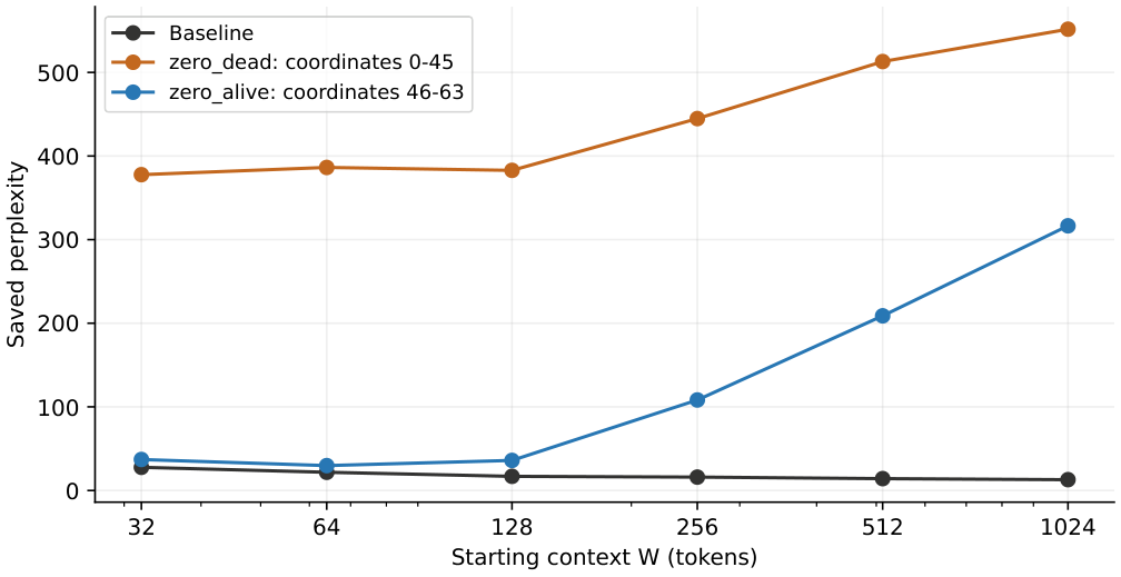
Full saved B3v2 window sweep. The curve labels identify coordinate masks, not semantic or positional channels. Points come from aggregate records; no uncertainty bars can be reconstructed from those aggregates.
The earlier B3 record tested passkey distances 50, 200 and 500: accuracy was zero in all three conditions. Its LAMBADA accuracies were \(0.005\), \(0\) and \(0.005\) for baseline, zero_dead and zero_alive, with \(n=200\); the stored PPL values were approximately \(454866\), \(283545\) and \(2038171\). These floor-level results cannot discriminate the proposed functions. They are retained separately from B3v2, rather than discarded or presented as corroboration. Both original JSON files accompany this revision.
13.3 The score simulation and the GPU amplification record
The historical score simulation used \(s(d)=\sum _k\sqrt{E_k}\cos (d\omega _k)\) and scaled a selected index group. It is not an attention probability model: learned Q/K phases, input-dependent coefficients and the causal softmax denominator are absent. Its original summary is retained below as a simulation report, with its historical index cutoffs. Those cutoffs are not the verified Pythia rotary-plane counts. Consequently, a simulated slope near zero after removing a group cannot validate a neural mechanism.
|
Model |
\(\theta \) |
cutoff |
old fit |
\(g(0)\) |
\(g(2)\) |
\(g(3)\) |
candidate |
|
Pythia-70M |
10K |
23 |
.748 |
.113 |
.484 |
.685 |
.752 |
|
Pythia-160M |
10K |
23 |
.511 |
.118 |
.474 |
.648 |
.752 |
|
Pythia-1B |
10K |
91 |
.931 |
.120 |
.423 |
.549 |
.752 |
|
SmolLM2-360M |
100K |
18 |
.969 |
.059 |
.210 |
.257 |
.972 |
|
Qwen2.5-0.5B |
1M |
15 |
1.028 |
.043 |
.218 |
.282 |
.997 |
Colour: blue shade = the number’s size within its column.
13.4 What the amplification code actually changes
The saved GPU panel contains four amplification settings on Pythia-70M. Re-fitting the stored mean-attention arrays reproduces its slopes and \(R^2\). The available script uses 50 prompts and sequence length \(d+200\), sampling the last query and key 199. Its uniform-causal null is therefore \(1/(d+200)\), with slope \(0.439001\) on its eight-point grid, not the E4 \(d+50\) null. The historical label “via E4” obscured this protocol difference.
|
\(\alpha \) |
measured fit |
\(R^2\) |
score simulation |
|
1 |
0.769227 |
0.986052 |
0.33 |
|
2 |
0.727302 |
0.981538 |
0.48 |
|
3 |
0.667649 |
0.971580 |
0.69 |
|
5 |
0.702202 |
0.906031 |
1.03 |
Colour: blue shade = the number’s size within its column.
There is a separate intervention error. The script treats fused NeoX rows as three contiguous model-wide Q, K and V blocks, but the actual layout is head, Q/K/V, coordinate. On a synthetic tensor with the configured dimensions, the function scales 276 Q rows, 230 K rows and 230 V rows per layer. Q heads 0–5 are affected, K/V heads 0–4 are affected, and heads 6–7 are untouched. In each affected component it selects the first 46 coordinates; Pythia-70M has only 16 rotary coordinates per head. This is neither a Q/K-only operation nor a rotary-only operation.
The observed changes relative to \(\alpha =1\) are approximately \(-0.041926\), \(-0.101578\) and \(-0.067026\). Their sign is opposite to the simulation’s increases \(0.15\), \(0.36\) and \(0.70\). The baseline being largest among four settings does not establish an optimum: no task-quality objective, local two-sided search or uncertainty is supplied, and the saved WikiText PPL entries are NaN. The claim that trained weights occupy a geometric optimum is withdrawn. Matching a configuration formula cannot repair the mask.
Output projection sparsity.
The former \(W_O\) experiment reported less than \(1.3\% \) throughput change after dense zeroing and a roughly sevenfold PPL increase on random tokens. These remain historical reports, not a validated frequency-pruning result. RoPE rotates Q/K, not V; the input coordinates of \(W_O\) therefore have no direct “dead RoPE band” assignment. Zero entries in an unchanged dense matrix do not imply a measured FLOP, latency or memory reduction. The suggested \(3.5\times \) projection saving and the mechanism attributed to Q-ROAR are not established by this record. A sparse backend, matched task evaluation and an explicit coordinate map would be separate experiments.
What a discriminating follow-up requires.
Read the rotary dimension and actual pairing, verify fused QKV layout, hold V and nonrotary coordinates fixed, and compare equal-size masks of complete planes with randomized controls. Record whether biases are intervened on. Use the same target positions across context windows and store per-example losses; measure positional and content tasks separately. Until those tests exist, the saved effects support coordinate sensitivity, not a semantic reservoir, double dissociation or safe band-pruning rule.
14 Attention Profiles, Weight Ratios and Circuit Hypotheses
14.1 A conditional reference distribution is not a circuit detector
For each query \(i\), choose a nonempty set \(J_i\) of past keys, excluding self if \(d^{-g}\) is used. Normalize observed and reference weights on the same set:
Positive retained observed mass is required. Report the excluded sink/self mass, query selection and fitting protocol. The per-head statistic is
with any averaging across queries stated explicitly. MaxEnt characterizes \(q\) under its specified constraint; it does not prove that \(q\) is attention with semantic content removed. A nonzero KL can result from sinks, local structure, masking or reference misspecification. A small KL does not identify the function of the value vectors. Neither statistic identifies an induction circuit without separate task and intervention evidence.
The former screening recipe used 50 prompts, a \(0.05\) threshold, and claimed fewer than \(15\% \) of heads were flagged across nine models. These are historical screening settings and reports, not validated sensitivity, specificity or a sixfold reduction in the cost of discovering circuits. The earlier \(0.1\) “SWA sink” threshold also has no calibrated causal interpretation. A window cannot truncate a sequence shorter than itself; the 4096-window Mistral configuration cannot explain a window-boundary effect in the short sequences examined here. A held-out labelled benchmark and matched masked/unmasked controls would be needed for a detection claim.
14.2 Weight-space measurements: coordinates and averaging
The saved spectral scripts group adjacent output coordinates over the full head dimension. The TransformerLens version uses columns of tensors stored as (head, input, output); the raw-Hugging-Face version uses rows of the linear-weight matrix. For a coordinate group \(I_k\), their Frobenius-product statistic is
This is a product of norms, not a variance-based signal-to-noise ratio. The inspected Pythia configs have partial RoPE and the inspected NeoX implementation uses split-half pairing. The archived full-head adjacent groups cannot be relabelled as true rotary planes by inverting their ratio. For TransformerLens exports, the conversion/permutation must additionally be verified; its historical version is not frozen in the experiment record.
Let \(a_{\ell h}\) and \(b_{\ell h}\) be the means of \(E_{\ell h k}\) below and above the archived cutoff. The saved summary is
In general neither equals the opposite-direction mean ratio or a ratio of grand means. For Pythia-1B, \(M_{\rm hist}=0.900342\), \(R_{\rm hist}=1.110689\), while the mean of \(b/a\) is \(1.113334\) and the ratio of group grand means \(a/b\) is \(0.894128\). For Pythia-70M, the corresponding \(M_{\rm hist}\) and grand-mean ratio are \(0.872883\) and \(0.800258\). The aggregation convention matters.
|
Model |
\(d_{\rm head}\) |
cutoff/groups |
\(M_{\rm hist}\) |
\(1/M_{\rm hist}\) |
grand ratio |
|
pythia-1.4b |
128 |
46/64 |
0.884877 |
1.130101 |
0.865139 |
|
pythia-1b |
256 |
91/128 |
0.900342 |
1.110689 |
0.894128 |
|
pythia-2.8b |
80 |
29/40 |
0.873084 |
1.145365 |
0.848381 |
|
pythia-410m |
64 |
23/32 |
0.874479 |
1.143538 |
0.803702 |
|
pythia-70m |
64 |
23/32 |
0.872883 |
1.145629 |
0.800258 |
|
SmolLM2-1.7B |
64 |
22/32 |
0.787101 |
1.270485 |
0.778233 |
|
SmolLM2-135M |
64 |
19/32 |
0.846094 |
1.181902 |
0.853030 |
|
SmolLM2-360M |
64 |
19/32 |
0.851445 |
1.174475 |
0.850211 |
Colour: blue shade = the number’s size within its column.
The table is recalculated from stored per-head ratios and averaged profiles; it is not a new weight measurement. The old Pythia-1B \(1.38\) and \(M=0.725\) do not describe this full-head record. The former 32-bar figure was also inconsistent with its caption of 16 heads: the stored full-head record has 16 layers, eight heads and 128 adjacent coordinate groups. Figure 14 now displays that record with coordinate labels and no semantic assignment.
🖼️ Figure 14
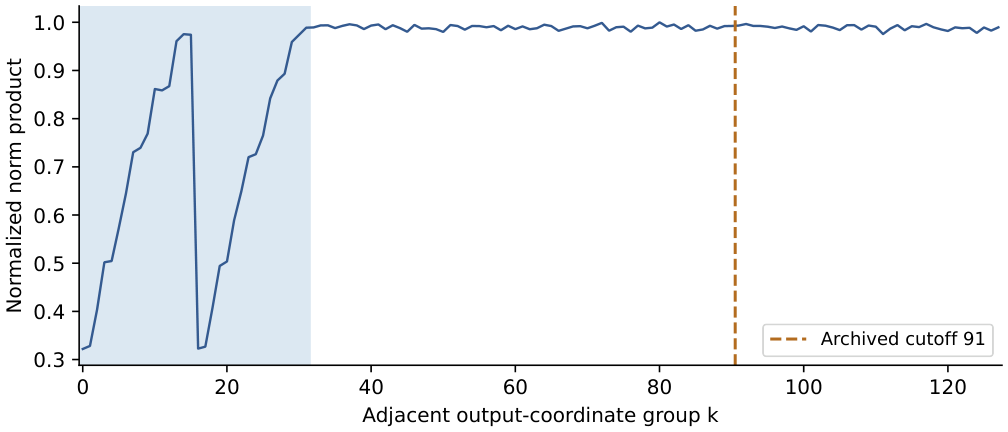
Saved Pythia-1B adjacent-coordinate norm-product profile, averaged over 16 layers and eight heads, normalized by its maximum. The shaded first 32 groups cover the 64 rotary coordinates in the native ordering; adjacent groups are not the split-half rotary planes. The dashed line marks the archived cutoff 91. Export-basis provenance remains necessary.
Other saved metrics must remain distinct.
The earlier squared-norm summary used a different formula, \(E_k=(\| W_Q[:,2k]\| ^2+\| W_Q[:,2k+1]\| ^2+ \| W_K[:,2k]\| ^2+\| W_K[:,2k+1]\| ^2)/(4d_{\rm model})\). Its reported rows are retained below with their original cutoff and group labels interpreted only as coordinate indices.
|
Model |
old cutoff |
first mean |
second mean |
old ratio |
|
Pythia-70M |
23 |
.0186 |
.0278 |
1.495 |
|
Pythia-160M |
23 |
.0067 |
.0096 |
1.437 |
|
SmolLM2-360M |
18 |
.0321 |
.0341 |
1.061 |
|
Qwen2.5-0.5B |
15 |
.0008 |
.0008 |
.980 |
Colour: blue shade = the number’s size within its column.
Those rounded energies do not determine all the printed ratios to three decimals. They cannot be substituted for the Frobenius-product panel. Similarly, the historical SVD summary reported \(k_{\rm obs}=21.5\pm 8.7\) and a contrast of \(1.03\). A claimed integer prediction \(2n=35\) cannot be twice an integer plane count; a continuous approximation would have to be identified as such and supplies no theorem linking cycles to singular-value energy coverage. The former \(38\% \) error and the geometric mechanism inferred from comparing different “SNR” quantities are withdrawn.
The two GQA aggregate records.
The separate Qwen file reports global ratios \(0.903216\) (0.5B) and \(0.880607\) (3B), while its layer-ratio means are \(0.883547\) and \(0.877954\). Their reciprocals reproduce the historical approximately \(1.107\) and \(1.136\) global values; these have a different aggregation path from the eight-model table. Two confounded observations establish neither absence of a GQA effect nor a universal shared mechanism. The exact input records and both aggregation conventions accompany this revision.
Correlations and the meaning of \(M\).
Across the five saved Pythia records, Pearson correlations with \(d_{\rm head}\) are \(r(M_{\rm hist},d_{\rm head})=+0.987556\) and \(r(R_{\rm hist},d_{\rm head})=-0.986580\). The latter is a strong negative sample correlation, not a weak or partial correlation. These five sizes do not control for architecture, training or the changed coordinate grouping. The historical multivariate expression \(1.13+0.0009d_{\rm head}-0.008\log _{10}\theta \) predicts \(1.3284\) for Pythia-1B, not its stored \(1.110689\); it is not retained as a fitted predictor. The five Pythia values of \(M_{\rm hist}\) range from \(0.872883\) to \(0.900342\), and the eight-model panel ranges from \(0.787101\) to \(0.900342\). Combining the two Qwen global ratios gives a heterogeneous ten-model range up to \(0.903216\), not \([0.72,0.90]\).
\(M\) denotes an explicitly defined coordinate norm ratio only. \(M=1\) is parity under that definition, not a reasoning/memory boundary, semantic capacity or fractal packing transition. The normalized architecture score \(\widehat M\) has no validated predictive baseline and is withdrawn as a comparison rule. Figure 15 retains the seven historical points, with corrected values and descriptive axes; its exponents and ratios come from different protocols and do not constitute an architecture taxonomy.
🖼️ Figure 15
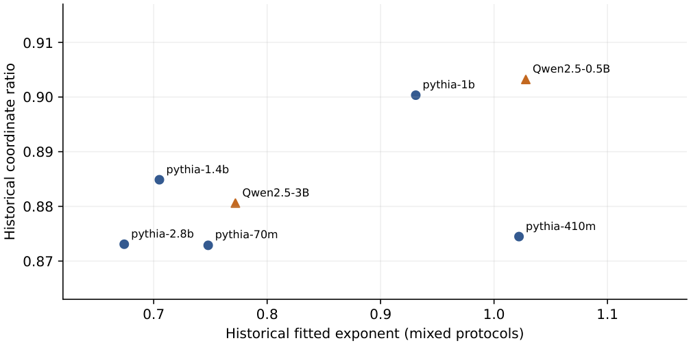
Seven historical exponent/coordinate-ratio pairs. Pythia uses the mean of per-head ratios; Qwen uses the separately saved global ratio. These are descriptive points with mixed provenance, not semantic scores. No phase regions or causal interpretation are assigned.
Software consistency.
The local tools/taf/diagnose/m_score.py is not an implementation of the archived statistic. It averages Q/K norms rather than multiplying them, uses a different complementary cutoff formula, and splits the fused NeoX tensor into three model-wide blocks. A synthetic row-identity check recovers only 256 of 2048 expected Q rows and none of the expected K rows for the 1B shape. It also omits the partial-rotary restriction. Its output must not be cited as a reproduction of these tables. This manuscript audit does not modify or certify the deployed software; source snapshots and the synthetic checks are included in the reproducibility package.
Extended historical exponent panel.
The 26-point map retains its historical panel, with the Pythia-2.8B contrast corrected to the matched 30–100 grid. Its cross-protocol and architecture claims require reconciliation with the row-level evidence; no induction threshold, SWA mechanism or controller prescription is inferred.
🖼️ Figure 16
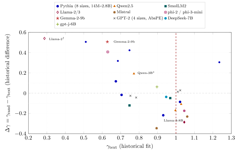
Historical 26-point exponent-difference panel, with the Pythia-2.8B contrast corrected from the unequal-support \(-.123\) to \(+.117\) on the common 30–100 grid (Section 8.4). Colors and markers group the series; the values combine historical protocols and are not circuit or architecture classifications. In particular, the plotted Qwen-3B difference is \(+0.192\); the former caption’s \(-0.225\) described a different comparison and must not be substituted for it. Dashed lines are reference values, not validated functional boundaries.
14.3 The \(\gamma \)-Field: Heterogeneity and Its Instrument Null
The available field extractor measures the last query at sequence length \(d+60\), always against key 59. It averages randomly generated token prompts at each distance, then fits each layer/head separately. This is neither the fixed-query October QL protocol nor the \(d+50\) E4 procedure. Its causal uniform profile is
Executing the actual extractor and fitter on synthetic causal-uniform matrices gives \(\widehat\gamma _0=0.755252\), \(R^2=0.985521\) on \(\{ 30,50,100,200,500,1000,2000\} \). With the six-point grid ending at 1000 the null slope is \(0.710309\). The five saved records use different prompt counts and, for 2.8B, a different grid; those settings are part of the observation, not interchangeable replications.
|
Pythia |
\(L\times H\) |
prompts |
\(d_{\max }\) |
global |
mean |
std |
NaN % |
|
1.4b |
\(24\times 16\) |
100 |
2000 |
0.690 |
0.907 |
0.463 |
4.688 |
|
1b |
\(16\times 8\) |
60 |
2000 |
0.753 |
0.943 |
0.331 |
0.781 |
|
2.8b |
\(32\times 32\) |
50 |
1000 |
0.969 |
1.309 |
0.631 |
0.195 |
|
410m |
\(24\times 16\) |
100 |
2000 |
0.979 |
1.328 |
0.602 |
37.500 |
|
70m |
\(6\times 8\) |
80 |
2000 |
1.122 |
1.579 |
0.817 |
37.500 |
Colour: blue shade = the number’s size within its column.
All five use seeds 42 and 123. Counts in the table are prompts per seed and distance. The JSON stores fitted matrices, not per-distance attention arrays or prompt-level outcomes. The means and standard deviations above are recalculated over finite fitted cells. The script accepts a head if at least three distance means are finite and exceed \(10^{-12}\); it applies no \(R^2\) acceptance threshold. A NaN marks failure of that numerical/data criterion, not an identified semantic head or failure of a power-law goodness-of-fit test.
Pythia-70M has 18 NaN cells: two in L3 and eight each in L4 and L5, using zero-based indices. L4–L5 alone account for \(16/48=33.3\% \), not the full \(37.5\% \). Pythia-410M also has \(37.5\% \) NaNs, all 16 heads of each layer L15–L23. This panel does not identify an induction threshold at 400 million parameters or establish \(L_{\rm crit}\) from missing fits.
The global fit is below the finite-cell mean in all five records. The distance-dependent mixture derivative in Section 10 explains why averaging slopes differs from fitting a mixture, but does not prove that these measured profiles are exact power-law components or that the reported global slope is an asymptotic tail exponent. The global nanmean also permits the participating head set to vary by distance. Head-specific null corrections would require each accepted support and weighting; the common null must not be subtracted indiscriminately from cells fitted on fewer points.
The outlier rule in the script is mean \(\pm 2\) standard deviations, not fixed thresholds of \(0.1\) and \(2\). For the 1B record, the saved high heads are (L0,H4) \(2.204\), (L1,H3) \(2.772\) and (L3,H0) \(1.810\), and the low head is (L1,H0) \(0.077\). The 2.8B record contains a maximum of \(7.389\) in L30,H0; L30 is penultimate, not the last attention layer. Flagging a head does not exclude it from the reported global fit or identify its task. The inverse association between head dimension and field dispersion is descriptive; it does not follow from a Riemann-sum argument or isolate training-induced specialization.
The four Pythia-1B training checkpoints.
|
Step |
global fit |
finite-cell mean |
std |
NaN % |
|
1 |
0.757234 |
0.757522 |
0.016958 |
0.000 |
|
1,000 |
0.851255 |
0.877925 |
0.213461 |
0.000 |
|
10,000 |
0.875856 |
0.885266 |
0.352252 |
0.000 |
|
143,000 |
0.717686 |
0.891705 |
0.338022 |
0.781 |
Colour: blue shade = the number’s size within its column.
These records use 100 prompts per seed and the same seven-point grid. The step-1 global slope \(0.757234\) is only \(0.001982\) above the matched uniform null. Thus its proximity to \(0.75\) is not evidence that a learned geometric attractor has already emerged. All four global slopes are below one: the \(0.875856\) checkpoint is not in the manuscript’s \(g{\gt}1\) regime. Finite-cell dispersion grows from \(0.016958\) to \(0.352252\) and then falls to \(0.338022\). This records heterogeneity under the stated estimator; it does not measure semantic capacity, overtraining or functional diversity without independent task evidence. The final \(0.717686\) checkpoint and the separate \(0.753024\) panel record have different prompt counts and should not be collapsed into a single exact value.
Token-class profiles: separate protocol and replay.
The saved Pythia-1B lexical experiment uses 50 prompts of length 1100 and fits distances \(30,50,100,200,500,1000\). It samples eligible queries from position 60 onward, unlike the last-query field extractor above. Its selection is strictly \(R^2{\gt}.5\), not \(R^2\ge .5\).
|
Class |
PUNCT |
COMMON |
MID |
RARE |
WHITESP |
NUMERIC |
|
Median \(g\) |
.612941 |
.754994 |
.651151 |
.853760 |
.830354 |
.921402 |
|
Selected cells |
50 |
39 |
47 |
32 |
92 |
113 |
|
Mean \(R^2\) |
.412156 |
.351339 |
.384916 |
.310053 |
.609364 |
.738798 |
The different averaging populations explain why mean \(R^2\) can be below the selection threshold. Class labels use decoded-token heuristics and token-ID cutoffs (COMMON below 1000, RARE above 30000), not measured corpus frequency bins. The number stored as total queries sums contributions across distances and heads; it is not a count of distinct independent queries. Selected head sets differ between classes, so their medians are not paired contrasts and do not establish multifractality.
Although context length is fixed, the eligible query pool changes with distance: a query \(q\) contributes only if \(q\ge d\). For uniform causal attention the class-specific mean is the average of \(1/(q+1)\) over that distance’s eligible class queries, and need not be flat. The saved fit matrices omit query positions and per-distance class counts, preventing an exact matched lexical-null reconstruction. These limitations also apply to interpreting the exploratory cross-family summaries. The median spread \(.921402-.612941=.308461\) is descriptive, not a measured geometric dimension or a critical fluctuation.
15 Base/Instruct Comparisons Under a Variable-Length Probe
15.1 Estimand, protocol and provenance
We use \(\delta \gamma =\widehat\gamma _{\rm instruct}-\widehat\gamma _{\rm base}\) for a checkpoint contrast. This is distinct from the random-minus-text corpus contrast \(\Delta \gamma \) in Section 16, and from a residual against \(\gamma _P\). The eight D3 pairs are retained as reported observations; they do not isolate reinforcement learning from SFT, DPO or other changes. An instruction checkpoint is not by itself evidence that RLHF was used.
The available cloud_d3_rlhf_kaggle.py specifies 50 random-token prompts per distance, seed 42, fp16 and eager attention. It generates lengths \(n=d+60\), reads the final query at key position 59 (zero-based), pools finite head/layer attention values, and fits OLS in log space at \(d\in \{ 30,50,100,200,500,1000\} \). Distances 10 and 20 are measured but not fitted. Uniform causal attention therefore yields
This is the matched D3 null, not the \(d+50\) E4 null. The actual fitting function and an independent 50-digit calculation agree. No new checkpoint inference was run. Subtracting this common null from both slopes leaves their difference unchanged; it does not remove model-dependent sinks, token effects or missing attention values.
The manuscript’s eight-pair table is the available D3 numerical summary. Its full d3_rlhf_results.json was not located in the searched local results and experiment directories. The instruct column and three base entries therefore retain rounded-manuscript provenance. Five base values have a recoverable numerical counterpart in the round-2 random-token arrays: SmolLM2-1.7B (\(0.866259\)), Qwen2.5-0.5B (\(0.906234\)), Qwen2.5-1.5B (\(0.980402\)), Qwen2.5-3B (\(0.746480\)), and Llama-3.2-3B (\(0.678947\)). All reproduce the D3 base entries after rounding to three decimals. The two available scripts share the random-token rule, \(d+60\), seed 42, 50 prompts, fit grid and fp16 setting for these models. This establishes reproducible counterpart values under matching declared protocols, but matching rounded values does not prove that D3 reused those exact runs. It does not reconstruct the missing instruct arrays or paired uncertainty. A separate April 21 two-pair JSON reports different values and remains a separate experiment. The script’s planned panel also contains a Phi-3 self-pair (the same checkpoint twice); that entry is not an independent base/instruct pair and is not included in the eight rows.
|
Pair |
base |
instruct |
\(\delta \gamma \) |
descriptive bin |
|
SmolLM2-135M |
0.913 |
0.922 |
\(+0.009\) |
small |
|
SmolLM2-360M |
0.890 |
0.887 |
\(-0.003\) |
small |
|
SmolLM2-1.7B |
0.866 |
0.916 |
\(+0.050\) |
increase |
|
Qwen2.5-0.5B |
0.906 |
0.848 |
\(-0.058\) |
decrease |
|
Qwen2.5-1.5B |
0.980 |
0.973 |
\(-0.007\) |
small |
|
Qwen2.5-3B |
0.746 |
0.698 |
\(-0.048\) |
decrease |
|
Llama-3.2-1B |
0.829 |
0.757 |
\(-0.072\) |
decrease |
|
Llama-3.2-3B |
0.679 |
0.730 |
\(+0.051\) |
increase |
Colour: blue shade = the number’s size within its column.
15.2 What the reported differences support
At the explicitly chosen descriptive cutoff \(0.02\), the correct counts are two increases, three decreases and three small changes. “Small” means \(|\delta \gamma |\leq 0.02\) in this table, not statistically indistinguishable or mechanistically unchanged. The largest reported absolute change is \(0.072\); no displayed pair crosses one. These are properties of eight rounded estimates, not bounds on post-training or evidence for a phase barrier. Opposite signs in the two Llama-3.2 pairs do not identify which recipe component caused either shift. A negligible scalar shift does not show that learning acted only on MLPs or output logits.
The script resets the random generator for each checkpoint. Identical token sequences within a pair additionally require equal tokenizer vocabulary bounds; the archived summary does not establish all tokenizer revisions. Across distances, the generator advances and the inputs differ. Per-prompt attention profiles and loss/task outcomes were not recovered for D3, so this audit cannot construct paired confidence intervals or assess whether the chosen cutoff exceeds sampling variability. No preregistration record or independent test set supports the former correlation and early-warning claims.
Consequences for monitoring.
The exponent can be recorded alongside loss and task metrics under an invariant instrument, but predictive monitoring requires prospective validation. The previous \(C_V{\gt}20\) catastrophic-forgetting alarm is withdrawn: at \(N=2000\) the finite-family maximum is approximately \(6.92\). Neither the eight pairs nor their size ordering establishes a \(4\times 10^8\) induction-head threshold, alignment quality, safety, or a universal post-training effect.
16 Corpus Contrasts and the Unvalidated Architecture Ratio
16.1 A descriptive statistic with a fixed sign convention
For a specified checkpoint, precision, attention implementation, distance grid and length/query rule, define
↳ Not used by another result of the paper.
En palabras.
El contraste resta el exponente ajustado en texto al ajustado en tokens aleatorios. Su signo solo se interpreta si se han emparejado checkpoint, precisión, implementación, malla de distancias y regla de consulta.
Alcance.
El signo no identifica por sí solo un circuito, una arquitectura ni una causa de la diferencia observada.
A positive contrast means a steeper fitted random-token profile and a flatter text profile on that support; a negative contrast means the converse. Neither sign identifies an architecture or an induction circuit. A residual against \(\gamma _P\) is a different quantity and must not be substituted here. Matching the instrument is necessary; it does not make corpora, tokenizers or training histories exchangeable across models.
16.2 Historical comparisons and architecture corrections
|
Model |
\(G\) |
window |
random |
text |
\(\Delta \gamma \) |
|
Gemma-2-9B |
2 |
4096 |
1.135 |
.628 |
+.507 |
|
Llama-3-8B |
4 |
– |
.931 |
1.046 |
-.115 |
|
Mistral-7B-v0.1 (fp16) |
4 |
4096 |
.830 |
1.061 |
-.231 |
|
Pythia-70M |
1 |
– |
.748 |
.748 |
\(\approx 0\) |
|
Falcon-7B (RoPE, MQA) |
71 |
– |
\(R^2\): .88 / .999 |
unavailable |
|
Colour: blue shade = the number’s size within its column.
The earlier comparison actually lists five model entries, not seven; Falcon has no pair of exponents in that table. These summaries are retained as a separate panel from the cloud rounds below. Pythia-70M’s duplicated \(0.748\) does not establish equality across corpora; the matched-grid analysis in Section 8.4 takes precedence for that comparison. Likewise Llama-3-8B values \(-0.287\), \(-0.115\) and \(-0.034\) appearing in different records are not repeat estimates under an established common protocol. Qwen2.5-3B’s \(+0.192\), \(-0.225\) and \(-0.053\) must not be merged into a single architecture signature. The record and its grid must accompany each value.
Google’s reference Gemma-2-9B configuration has 16 query heads, 8 KV heads, \(d_{\rm head}=256\), and an alternating local/global pattern with local window 4096; thus \(G=n_q/n_{\rm kv}=2\), not 8. 1 Falcon-7B uses RoPE and multi-query attention, rather than ALiBi, as recorded in the configuration audit. Mistral-7B-v0.1’s configured window is also 4096. For sequences of at most 2050 tokens in the earlier E4 panel, or 1060 tokens in the cloud protocol, a 4096-token local mask excludes no additional causal keys. Therefore an active sliding-window cutoff cannot explain these measured differences. Training with local attention could still affect the learned weights; that separate hypothesis was not tested by these comparisons.
The old sign-based decision tree and the claim that configuration files can be replaced by two scalar fits are withdrawn. Architecture should be read from the exact configuration and implementation. Circuit identification needs behavioral and intervention evidence, such as the small-model experiments of olsson2022induction; their work does not supply a universal \(4\times 10^8\)-parameter threshold.
16.3 Cloud rounds: shared estimator, different evidence depth
The round-2 and round-3 scripts use 50 prompts, seed 42, the \(d+60\) rule and the same six fitted distances as D3. They compare random IDs with contiguous WikiText-2 training-text chunks, averaged across finite head/layer values. Text chunks are sampled anew by length; random and text prompts are not paired semantic counterparts. Precision varies by model, and round 4 uses 4-bit NF4 for Mistral. The matched uniform null is again \(0.7103091963\).
There is an additional provenance hazard: the round-2/3 text-loading failure path reuses the random result as “text”. That branch forces \(\Delta \gamma =0\) without measuring text. We do not claim it occurred in the successful rows below, whose corpus estimates differ; future outputs must record corpus-load success explicitly and treat fallback as missing, rather than neutral.
The archive provides full distance means for six successful round-2 models and Mistral in round 4. All fourteen corpus fits and their \(R^2\) values replay to numerical precision. Round 3 provides rounded summaries for Pythia-2.8B, Llama-3-8B and a repeat of Llama-3.2-3B. The last is not counted as a new model. For Llama-3-8B the displayed \(0.821-0.856=-0.035\), while the saved rounded contrast is \(-0.034\); we preserve the latter as reported, without inventing unavailable digits. Failed loads and incomplete models are not measurements.
16.4 Recomputing the proposed ratio
The historical heuristic was
Here \(N_0\) is a chosen reference scale, not an established induction threshold. The numerator is not the GQA sharing factor \(n_q/n_{\rm kv}\) and is not a measured channel capacity. The mathematical ratio is singular at \(N=N_0\); the archived helper additionally returns NaN for \(N\leq N_0\) or \(n_{\rm kv}\geq d_{\rm head}\). Those software restrictions are not physical boundaries. The previous MHA example incorrectly dropped \(n_{\rm kv}\): with \(d_{\rm head}=64\), eight KV heads and \(N=10^9\), the ratio is \(\log 8/\log 2.5\simeq 2.269\), not \(\log 64/\log 2.5\simeq 4.539\).
|
Model |
round |
\(R_c\) |
random |
text |
\(\Delta \gamma \) |
\(R^2_{\rm rnd}\) |
|
pythia-2.8b |
3 |
0.473 |
0.810 |
0.769 |
\(+0.041\) |
0.961 |
|
SmolLM2-1.7B |
2 |
0.479 |
0.866 |
0.846 |
\(+0.020\) |
0.997 |
|
Llama-3-8B |
3 |
0.924 |
0.821 |
0.856 |
\(-0.034\) |
0.966 |
|
Mistral-7B (NF4) |
4 |
0.957 |
0.834 |
0.981 |
\(-0.147\) |
0.678 |
|
Yi-6B |
2 |
1.275 |
0.966 |
0.842 |
\(+0.124\) |
0.980 |
|
Llama-3.2-3B |
2 |
1.331 |
0.679 |
0.594 |
\(+0.085\) |
0.942 |
|
Qwen2.5-3B |
2 |
2.034 |
0.746 |
0.799 |
\(-0.053\) |
0.988 |
|
Qwen2.5-1.5B |
2 |
3.085 |
0.980 |
1.063 |
\(-0.083\) |
0.959 |
|
Qwen2.5-0.5B |
2 |
17.078 |
0.906 |
0.861 |
\(+0.045\) |
0.991 |
Colour: blue shade = the number’s size within its column.
Table 34 uses the scripts’ nominal parameter counts and head metadata; it does not certify exact parameter totals from every checkpoint. The failed Gemma row’s archived \(n_{\rm kv}=16\) is incorrect (the reference configuration has eight), and is not promoted into a successful observation. The two corpus fits for Mistral are \(0.834184\) and \(0.981382\), giving \(-0.147198\), but the random-token \(R^2\) is only \(0.677965\). Its random profile is nonmonotonic, including a large distance-100 value. It is thus especially weak evidence for a power-law signature. Its difference from the older fp16 contrast \(-0.231\) is not a controlled quantization effect.
16.5 What fails, and what remains untested
Using the sign of the nine reported contrasts, the minimum–maximum ranges are
Their interval intersection is \([0.924358,3.085057]\). This is an intersection of two sample range hulls, not a densely measured zone, confidence interval, phase boundary or evidence that every point in it supports both signs. The previous intervals \([0.4,1.0]\), \([0.47,1.33]\) and \([0.5,1.3]\) do not represent that calculation. Classification cutoffs also changed historically between zero, \(0.02\) and \(0.1\); they must not be mixed. Here signs are descriptive and no “pre-IH” or “post-IH” ground-truth labels are assigned.
The statement “all models with \(R_c\geq 2\) have negative contrast” is false: Qwen2.5-0.5B has \(R_c=17.077567\) and \(\Delta \gamma =+0.044788\). Its proximity to the chosen singular reference scale explains sensitivity of the ratio, not permission to remove the counterexample after seeing it. Llama-3-8B and Mistral have negative contrasts below one, while Pythia-2.8B and SmolLM2-1.7B have positive contrasts there. These selected heterogeneous models do not establish a monotone rule or a causal effect of KV sharing.
At fixed \(d_{\rm head}\) and \(n_{\rm kv}\) with positive numerator and \(N{\gt}N_0\),
Thus the earlier advice to raise \(N\) to raise \(R_c\) was algebraically reversed. Lowering \(n_{\rm kv}\) does raise this ratio, but the archive does not show that doing so improves induction, quality, safety or training efficiency. The ratio-based architecture prescriptions and their \(\alpha _S\) extension are withdrawn; Appendix H preserves their definitions and examples as an unvalidated historical construction.
An adequate follow-up would pin checkpoint/config/tokenizer/library revisions, hold precision and contexts fixed, record per-sequence profiles and corpus-load status, and compare candidate decay families on held-out sequences. Confidence intervals should resample sequences, not treat heads or distances as independent replicates. A causal KV-head claim additionally requires a controlled architectural intervention and direct circuit/task outcomes. Neither a sign contrast nor a good in-sample log–log fit supplies those tests.
17 Diagnostic Manual and Model Encyclopaedia
Revision of 7 November 2026
The model encyclopaedia and command examples remain for continuity. Their configuration, measurement and recommendation fields must be distinguished. Do not fill a missing measured exponent with a configuration formula or treat a historical “safe”/“requires NTK” verdict as a current recommendation. The software interface and model metadata may have changed; this revision does not assert that all printed commands or current remote outputs were retested.
17.1 Using the archived diagnostic CLI
The November 5 snapshot contains cli/diagnose_model.py. Its example command, relative to that software checkout, is
python cli/diagnose_model.py --model EleutherAI/pythia-70m --fast --cpu
The inspected snapshot defines four fast distances \(10,50,200,1000\) and 30 attempted prompts per distance, not 20. Full mode attempts 80 prompts per distance on the nine-point grid
Successful fits depend on available attention outputs and valid samples. Its recorded protocol uses lengths \(d+50\) and the final query, so the matched-null cautions apply. Runtime, CPU memory and model support depend on the actual checkpoint, libraries and hardware; the old three-/fifteen-minute universal promises are withdrawn. Quantization is an optional backend with its own requirements, not a guarantee for every model above a size threshold. Printed commands are source documentation, not commands executed in this audit.
17.2 Measurement Decision Guide
Record the exact checkpoint/configuration, tokenizer, precision, attention implementation, corpus, length/query rule, seeds, distance support and aggregation. Compute a matched null through the same estimator. Fit alternative decay families and inspect residuals on held-out sequences; a low power-law \(R^2\) does not identify ALiBi or SWA. Report corpus contrasts without mapping their signs to architectures.
|
Observation |
Follow-up |
|
Poor power-law fit |
Inspect support, masks, sinks and competing families; do not infer architecture from \(R^2\). |
|
Fit near or above one |
Compute finite-support quantities; validate any cache policy with task outcomes. |
|
Nonzero corpus contrast |
Preserve both estimates and their uncertainty; check matched metadata and corpus-load success. |
|
Head or layer heterogeneity |
Inspect individual profiles; establish circuit function with direct tests. |
|
Large mass quantile |
Treat as a distributional calculation, not a guarantee of useful retained context. |
The previous threshold flowchart is superseded by this measurement-first guide; its exact text and diagram source remain in the revision archive.
17.3 Architecture Design: Withdrawn Scalar Prescriptions
The earlier five-step tree mapped task names to target exponents, inverted \(\gamma _P\) for a RoPE base, required \(R_c\geq 2\), and used \(\alpha _S\) to decide whether to train. These prescriptions are withdrawn. The cloud panel contains a positive-contrast model above \(R_c=17\); the claimed induction threshold is not established; and raising model size lowers the written ratio under its usual positive-domain assumptions (Section 16.4). An algebraic inverse of a candidate fit is not a validated architecture controller.
Choose context, memory, latency and quality requirements explicitly, then compare actual implementations on representative held-out tasks. A pilot should measure uncertainty and compare a baseline before selecting KV sharing, RoPE scaling or a cache policy. These measurements cannot be replaced by a scalar “ignition” score.
The associated hardware proposal also lacks support from the archived band ablations: their masks do not select complementary rotary-plane classes and one implementation changes V (Sections 14.2 and 13.4). The historical estimates of 25% attention compute and 7–15% total energy savings are proposals, not measured kernel speedups or quality-preserving guarantees. Correct plane indexing, an implemented sparse kernel and end-to-end quality/throughput measurements would be needed.
17.4 Model lookup with explicit calculation domains
Table 36 uses the 21 current panel identifiers rather than mixing obsolete gamma values, unverified precision labels and hardware recommendations. Each row stipulates a power family on \(1,\ldots ,2000\); this extrapolation is not a new attention measurement. To make the lookup exactly reproducible, the inputs are the six-decimal displayed exponents of Table 10. The discrete column is the smallest integer capturing at least \(.9\) of that family’s mass; the continuous column uses Lebesgue measure on \([1,2000]\). Neither is a quality-preserving cache prescription.
|
ID |
Model |
input \(g\) |
discrete |
continuous |
|
P01 |
phi-3-mini (text) |
0.629563 |
1527 |
1532.07 |
|
P02 |
Falcon-7B |
0.924685 |
1070 |
1106.76 |
|
P03 |
CodeLlama-13B |
0.382302 |
1689 |
1689.14 |
|
P04 |
Gemma-2-9B (text) |
0.627646 |
1529 |
1533.78 |
|
P05 |
Mistral-Nemo-Instruct |
0.428448 |
1667 |
1667.50 |
|
P06 |
Pythia-2.8B |
0.674162 |
1482 |
1489.31 |
|
P07 |
Pythia-1.4B |
0.705073 |
1447 |
1456.02 |
|
P08 |
SmolLM2-135M |
0.747996 |
1392 |
1404.20 |
|
P09 |
Qwen2.5-3B |
0.772033 |
1358 |
1372.05 |
|
P10 |
Pythia-70M |
0.747602 |
1392 |
1404.70 |
|
P11 |
SmolLM2-360M |
0.969173 |
963 |
1008.40 |
|
P12 |
Pythia-1B |
0.931108 |
1055 |
1093.12 |
|
P13 |
Qwen2.5-7B |
0.996695 |
892 |
943.26 |
|
P14 |
Qwen2.5-0.5B |
1.028374 |
807 |
864.95 |
|
P15 |
Mistral-7B-v0.1 |
1.060750 |
717 |
782.24 |
|
P16 |
Llama-3-8B |
1.045476 |
760 |
821.52 |
|
P17 |
Gemma-2-9B (random) |
1.134796 |
515 |
591.04 |
|
P18 |
phi-3-mini (random) |
1.036602 |
784 |
844.14 |
|
P19 |
Llama-2-7B (Kaggle) |
1.210761 |
334 |
410.37 |
|
P20 |
Llama-2-13B (Kaggle) |
1.054530 |
735 |
798.28 |
|
P21 |
BLOOM-7b1 |
1.217824 |
319 |
395.16 |
Colour: blue shade = the number’s size within its column.
The previous 14-row catalogue, including its unsupported recommendations and inconsistent model configurations, is preserved verbatim in the replacement log and predecessor PDF. Pythia-14M and OLMo values from other records are not silently substituted into this identified 21-row panel. Position schemes alone do not choose an empirical decay family: compare power, exponential and mixed alternatives on the actual support.18 Limitations and Open Questions
Revision of 7 November 2026
The original limitations, tables and failure atlas are retained, with additional limits stated locally. The Phase-A-only restriction on the finite continuous quantile is corrected: it is finite for all real \(\gamma \), with \(N^f\) at one. The main withdrawn claims are the geometric derivation of the learned exponent, independent inverse-horizon validation and task guarantees from mass alone. The 17 missing October observations and incomplete weight provenance are unresolved. The additions reuse saved evidence and do not repair it by inference.
We list the principal limitations of the framework honestly and in one place.
L1: the proposed geometric derivation is not established.
The power-law family follows conditionally from a log-distance score or a prescribed MaxEnt constraint; rotary cycle counts alone imply neither. The Padé candidate has no accepted universal derivation. Selected-panel error percentages do not repair its invalid boundary conditions or nonlinear averaging step (Appendix B).
L2: position scheme is not an empirical family diagnosis.
GPT-2 has absolute positions; BLOOM has ALiBi; Falcon-7B has RoPE/MQA. The finite power-family quantile is mathematical for any exponent, conditional on that family. No positional encoding by itself validates the family or a task-level cache or context-extension guarantee.
L3: coordinate effects do not establish frequency-specific functions.
The revised Sections 13 and 14.2 separate the B3 masks, GPU amplification, coordinate pruning and norm-ratio statistics. The historical B3 labels are not complete-plane interventions; its two masks affect different numbers of coordinates. The amplification script also changes V and leaves heads untouched. The full-head spectral summaries do not isolate the partial rotary subspace. Their effects and correlations therefore cannot validate a semantic reservoir, a geometric optimum or safe pruning. The original \(1.38\) and \(0.87\) labels must not be merged with the audited 1B \(M_{\rm hist}=0.900342\) and its reciprocal \(1.110689\). No new model run is claimed by the synthetic tensor checks or aggregate replays.
L4: base/instruct evidence is limited.
The eight-pair D3 manuscript summary has two increases, three decreases and three small changes at cutoff \(0.02\) (Section 15). Its raw output was not located; the available script gives the matched uniform null \(0.710309\). An earlier two-pair JSON is separate evidence. These observations do not isolate RLHF or validate attention-based warnings of forgetting or alignment changes.
L5: mathematical scope versus empirical use.
The finite continuous mass quantile applies to every real exponent, with \(N^f\) at one. The \(g{\lt}1\) large-\(N\) approximation can be inaccurate near one. A mass quantile does not guarantee task quality, and the variable-length E4 instrument produces a nonzero slope even for uniform attention.
L6: saved KV, base-scaling and retrieval experiments.
The complete two-model and seven-model B2 panels remain separate in Section 11. They test asymptotic windows with different target blocks and do not validate a universal favorable exponent interval. The B1 experiments below change a nominal RoPE base before loading the same weights; they do not fine-tune those weights. Their \(\alpha \) denotes the base multiplier, not the context-extension factor of every method called NTK scaling.
EXP-B1v3: long-sequence PPL and its denominator.
The saved Pythia-1B record has four base settings and four 64-token target bands, indexed from zero as \([960,1024)\), \([1984,2048)\), \([3008,3072)\) and \([4032,4096)\). The script requests up to ten 4096-token WikiText-2 test segments and supplies the whole prefix up to each band’s end. Thus 4096 is sequence length, not the number of sequences. The JSON preserves aggregate PPL, not per-sequence losses or immutable execution metadata. Pythia-1B was trained at 2048: bands A and B end within that context, whereas C and D test extrapolation. Their very large unscaled losses are not an in-context compression baseline.
|
\(\alpha \) |
PPL A |
PPL B |
PPL C |
PPL D |
B/A |
C/A |
D/A |
|
1 |
11.949 |
12.659 |
620.950 |
1424.147 |
1.059 |
51.966 |
119.183 |
|
4 |
13.878 |
14.549 |
16.084 |
12.366 |
1.048 |
1.159 |
0.891 |
|
16 |
40.117 |
59.789 |
72.969 |
77.539 |
1.490 |
1.819 |
1.933 |
|
64 |
79.969 |
143.510 |
172.836 |
219.855 |
1.795 |
2.161 |
2.749 |
Colour: blue shade = the number’s size within its column.
The historical ratios divide each setting’s B/C/D PPL by its own A PPL. They compare different target bands and suppress changes in the denominator. At \(\alpha =4\), A rises from 11.949197 to 13.877564 (\(+16.14\% \)), and B from 12.659133 to 14.549244 (\(+14.93\% \)), compared with \(\alpha =1\) on the same band. Its C and D PPL are much lower than the unscaled values. This is a recorded short/long-context tradeoff, not cost-free extension. The historical \(1.80\times \) at \(\alpha =64\) is B/A within that setting; B is instead \(11.34\times \) the unscaled B value. No paired uncertainty can be recovered from these aggregates.
The value 64 comes from clipping the legacy expression \(e^{\log (10000)/0.5}/10000=10000\) at 64. It is neither the inverse-candidate value \(0.434446\) at \(T=2048\) nor a demonstrated optimum. The data contain no fine-tuning test that could validate this prescription after weight adaptation. YaRN uses a different schedule and attention rescaling peng2023yarn; its results do not certify this base multiplier.
Earlier B1 protocols remain distinct.
The v2 PPL script crops 124, 148 or 150 context tokens plus 64 target tokens and supplies no offset position IDs: its inputs are only 188–214 tokens long. The large source-text offsets therefore do not test long positional contexts. All 20 v2 PPL aggregates are preserved in the evidence package. The original NIAH record contains 25 cells of \(0/40\) at five lengths and five base settings. Its next-token argmax criterion, comparing only the first token of each separately tokenized key, differs from the subsequent candidate-ranking task; the zero counts are retained, not discarded as failed measurements or pooled with v4/v5.
EXP-B1v4/v5: deterministic candidate-ranking NIAH.
The scripts score a correct numeric key against nine distractor entries in repeated laboratory-themed filler. The 50 insertion fractions form a fixed grid from 0.1 to 0.9; they are not random needle positions. Keys and distractors are selected deterministically from a tokenizer-filtered pool. A tie with a distractor counts as failure. This is restricted candidate ranking, not free-generation retrieval or reasoning. The model records retain historical exponent tags \(.748\), \(.931\), \(.705\) and \(.674\) for Pythia-70M, 1B, 1.4B and 2.8B, respectively. The v5 retrieval script does not remeasure these exponents after changing the base.
A reconstruction using the frozen local Pythia-70M tokenizer produces 75 pool entries but only 61 distinct keys; the first 50 trials use 42 distinct keys, and some trials have eight distinct distractors among the nine entries. The pool builder does not deduplicate and only uses its three-digit fallback if fewer than 20 entries were found. All reconstructed context lengths are \(L+1\) because BOS is added after the filler budget; scoring adds the key token as well. These are properties of the saved code with the specified tokenizer snapshot, not proof of the exact historical runtime. The aggregate JSON omits the token IDs, runtime frequency buffers, per-trial scores and immutable library/weight revisions needed for that stronger claim.
The plotted \(10\% \) line is the nominal reference for ten exchangeable candidate entries. Deterministic, duplicated and differently frequent keys do not establish that reference as the model’s measured no-needle accuracy. No matched no-needle or shuffled-label control is saved here. Reused keys and filler also prevent treating the 50 trials as independent corpus samples. We report counts without manufacturing paired significance from aggregates.
|
\(\alpha \) |
512 |
1024 |
2048 |
3072 |
4096 |
|
1 |
88 |
92 |
92 |
88 |
10 |
|
4 |
88 |
90 |
90 |
88 |
86 |
|
8 |
88 |
84 |
88 |
88 |
88 |
|
16 |
74 |
84 |
82 |
82 |
84 |
Colour: blue shade = the number’s size within its column.
|
Model |
\(\alpha \) |
512 |
1024 |
2048 |
3072 |
4096 |
|
pythia-70m |
1 |
88 |
92 |
92 |
88 |
10 |
|
4 |
88 |
90 |
90 |
88 |
86 |
|
|
8 |
88 |
84 |
88 |
88 |
88 |
|
|
16 |
74 |
84 |
82 |
82 |
84 |
|
|
pythia-1b |
1 |
100 |
100 |
100 |
16 |
16 |
|
4 |
100 |
100 |
100 |
100 |
100 |
|
|
8 |
100 |
100 |
100 |
100 |
100 |
|
|
16 |
100 |
100 |
92 |
90 |
88 |
|
|
pythia-1.4b |
1 |
100 |
100 |
100 |
16 |
12 |
|
4 |
100 |
100 |
100 |
100 |
100 |
|
|
8 |
100 |
100 |
100 |
100 |
100 |
|
|
16 |
100 |
100 |
98 |
98 |
98 |
|
|
pythia-2.8b |
1 |
100 |
100 |
100 |
16 |
24 |
|
4 |
100 |
100 |
100 |
100 |
100 |
|
|
8 |
100 |
100 |
100 |
100 |
100 |
|
|
16 |
100 |
100 |
100 |
100 |
100 |
Colour: blue shade = the number’s size within its column.
All 80 v5 cell counts reproduce their stored accuracies; the 20 v4 cells equal the v5 Pythia-70M panel exactly and are not counted as independent replication. At nominal \(L=4096\), unscaled accuracies are \(10,16,12,24\% \); at \(\alpha =4\) they are \(86,100,100,100\% \). At \(\alpha =8\) they are \(88,100,100,100\% \). The three larger models reach \(50/50\) under both 4 and 8; this observed ceiling is not a guarantee of population accuracy.
There is no strict Pareto dominance by \(\alpha =4\): on Pythia-70M it loses two percentage points against \(\alpha =1\) at both 1024 and 2048, and at 4096 it trails \(\alpha =8\) by two points. The \(\alpha =16\) Pythia-2.8B row remains at \(100\% \) at every tested length, contradicting a universal over-extension failure at 16. The large unscaled drops do not by themselves identify rotary aliasing as their cause. They support the recorded restricted-task comparison, not an exponent-derived optimum, a universal safe interval, or the threshold \(L^c=2d_{\rm inv}\).
figureSaved candidate-ranking accuracies for Pythia-70M (EXP-B1v4; 50 deterministic trials per cell). The v5 small-model panel is identical. Coordinates retain every reported value; \(\alpha \) is a base multiplier. The nominal ten-candidate reference is not a measured no-needle baseline. At \(L=4096\), \(\alpha =4\) scores \(43/50\) and \(\alpha =8\) scores \(44/50\). At 1024 and 2048, \(\alpha =4\) scores \(45/50\) versus \(46/50\) unscaled. These observations do not prove a universal optimum or an aliasing mechanism.
L7: the finite-family heat capacity is not sampling-temperature response.
nakaishi2024critical study correlations and critical behavior in generated text as the token-sampling temperature varies. That work does not establish the negative heat-capacity claim formerly attributed to it here; the attribution is withdrawn. Its sampling variable and observables differ from the fixed-support distance family used in this manuscript.
Our finite-family quantity is
It is nonnegative and finite for every real exponent at fixed finite \(N\). Only for fixed \(\gamma {\gt}1\) does the infinite-support normalizer tend to \(\zeta (\gamma )\); in that limiting family \(C_V\) diverges as \(\gamma \to 1^+\). For \(N=2000\), the positive-exponent finite maximum is instead near \(\gamma =1.256885\), with \(C_V=6.919812\). The factor \(\gamma ^2\) is essential: variance alone is Fisher information, not heat capacity. None of these identities supplies the response of token sampling or a physical transition in a trained model.
L8: mixture-of-experts needs architecture-specific definitions.
An expert need not own a separate attention operator. For example, Mixtral’s experts are feedforward blocksmixtral2024audit. A per-expert attention exponent therefore cannot be assumed from the term MoE. Routing-conditioned profile comparisons would need explicit query populations and controlled measurements; the inverse candidate does not validate a per-expert horizon.
L9: a single fitted exponent loses heterogeneity.
The field measurements in Section 14.3 retain head/layer variation and missing fits. A global family is a modeling choice. High family heat capacity need not occur exactly at one, and neither a fitted exponent nor a proxy gate establishes a head’s task sensitivity. Direct interventions and paired outcomes remain necessary.
L10: the original falsification claims do not survive this audit.
The proposed universal geometric predictor already fails the initial mixed-panel comparison and does not reproduce the October QL comparison. Those observations do not satisfy the earlier claimed five-percent error criterion. The E4 null also shows that a fitted power law does not require rotary geometry. Comparing different model families cannot isolate the effect of replacing a positional encoding; such a causal test needs matched training and measurement controls.
A negative relation between \(g\) and entropy computed from the same positive-\(g\) finite family is algebraic: \(\mathrm{d}H/\mathrm{d}g=-g\operatorname {Var}(\log d)\). It is not an independent empirical test of a physical entropy mechanism. The appropriate empirical objects are measured distributions, intervention effects and held-out predictions, with their uncertainty and controls.
Open questions.
(0) Forgetting and family heat capacity. At fixed finite \(N\), \(C_V\) does not diverge at one. On the positive-exponent family at \(N=2000\), the numerical maximum is approximately \(6.919812\) near \(g=1.256885\); the former threshold \(C_V{\gt}20\) is not an operative threshold in that setting. A slope change of \(0.05\) per epoch is also an unvalidated warning rule, especially when the estimator itself is context-dependent. No independent empirical corroboration of that proposed warning rule is established. Testing a warning rule requires matched checkpoints and predefined outcomes on held-out tasks, not coefficient or terminology matching.
(1) The initial panel has a Pythia-31M random estimate \(1.539824\); it does not support the former upper cap of \(1.35\). A cross-model empirical maximum would in any case depend on the acquisition protocol and selection of models.
(2) The EXP-D1 modular-addition pilot has 150 saved checkpoints. Its fitted gamma ranges from \(.319592\) to \(.456514\), always below one. Validation accuracy first exceeds \(.90\) at step 3400 and \(.95\) at step 3500; the latter threshold defines the reported grokking step, not a uniquely located transition. The probe uses four-token random sequences and only distances 1, 2 and 3, averaging different query pools at each distance. Three points do not establish an asymptotic attention tail. The saved field called \(C_V\) is actually \(1/|1-g|\) (with a cap), not the finite-family heat capacity. Thus the record does not support a crossing of one, but also does not identify an intra-phase circuit restructuring or settle a long-context grokking mechanism. The training model has learned absolute positions, not RoPE.
(3) Predicting forgetting from an inverse-coordinate score remains untested. (4) A relationship between vocabulary-rank and attention-distance exponents requires matched observables and controls; no exact duality is established.
L11: downstream validation remains restricted.
The saved cache and base-scaling experiments use WikiText-2 PPL and restricted numeric-key ranking. Neither validates multi-step reasoning, a universal cache exponent interval or an optimum for a target exponent. PPL measures predictive loss on the specified tokens, not coherence as an independent semantic outcome. Effects on math, code and long-document QA remain open; discarded attention mass alone does not predict their accuracy loss.
L12: no controlled MoE validation.
A saved OLMoE-1B-7B-0924 random-token E4 record does exist, so the former claim that no MoE profile was collected is incorrect. It is not a matched dense/MoE intervention study or an expert-conditioned analysis and does not validate a MoE extension of the horizon proposal.
L13: ALiBi bias is not the complete attention profile.
A linear negative-distance score bias contributes an exponential factor before normalization. Content scores, masks and numerical precision still matter. The historical BLOOM-1b7 zero at distance 5000 cannot by itself distinguish underflow, masking and very small positive mass. The exponentially cut-off family is a conditional mathematical model; its adequacy for ALiBi must be measured, not inferred solely from the position scheme.
L14: no established SGD-to-candidate attractor.
The constrained maximum-entropy result fixes a family after prescribing its log-distance moment; it does not determine which exponent SGD will learn. The rational-coordinate trajectory in Section 20 is not an observed optimizer trajectory. Neither a training attractor nor convergence to the configuration-based candidate follows from the saved pilot. The required dynamical bridge remains unproved.
L15: controlled-base pilot, instrument and training-objective audit.
The saved pilot contains three runs of a 4-layer GPT-NeoX-style transformer, with hidden size 128, four heads, head size 32, full rotary dimensions and 13,659,136 parameters. The code requests the same seed 42, initialization procedure, random-crop ordering and AdamW settings, while changing the base among \(10^4,10^5,10^6\). It sets both legacy and newer base configuration fields. No saved runtime frequency-buffer check or immutable library revision is available to certify their historical interpretation.
The script caps the WikiText-2 training stream at 2,000,000 tokens and requests 4000 steps of eight 512-token crops: 16,384,000 scheduled input-token presentations, with reuse. This is not one million training tokens or 2.4 million distinct corpus tokens. Nonfinite losses can skip steps and AMP can skip updates, so the schedule is not a verified optimizer-update count. The nine logged losses per run end at 6.466924, 6.475903 and 6.480629. These training losses are not held-out perplexities or convergence certificates.
Target-alignment defect in the saved script. Crops already set \(y_t=x_{t+1}\) and call the causal language model with labels=y. The standard causal loss shifts labels internally, pairing the logit at \(t\) with \(y_{t+1}=x_{t+2}\) instead of \(x_{t+1}\). Inspection of the installed Transformers 5.13.0 source and a synthetic-logit loss check verify this composition; no model forward pass is required. The historical runtime is not pinned, so this establishes a defect of the available recipe under that loss convention, not a reconstructed execution trace. The same internal shift also appears in the older public implementation. 2 The pilot cannot be certified as standard next-token pretraining without resolving this mismatch.
Measurement protocol. The extractor uses 30 crops for each distance \(d\in \{ 10,20,30,50,100,200,300,500\} \), with sequence length \(d+5\), all layers and heads, and the last query at distance \(d\). It reuses the training stream; lengths range from 15 to 505, rather than a fixed evaluation length 512. The candidate is nevertheless evaluated at \(T=512\). This is distinct from the earlier E4 protocol. The three per-base files match the combined JSON, and all slopes and fit scores below are replayed from eight saved means.
|
\(\theta \) |
\(\gamma _P(512)\) |
\(\widehat\gamma \) |
\(R^2\) |
rel. error (%) |
|
10000 |
0.930122 |
0.977318 |
0.996753 |
5.074 |
|
100000 |
0.992785 |
0.959179 |
0.996762 |
3.385 |
|
1000000 |
0.999276 |
0.959578 |
0.996552 |
3.973 |
Colour: blue shade = the number’s size within its column.
For uniform causal attention, the same selected entry equals \(1/(d+5)\). Fitting that null on the eight distances gives \(\widehat\gamma _0=0.9103752731\) and \(R^2=0.9978936065\). Consequently, a power fit above \(.99\) and a slope near one do not establish learned geometric organization. The excesses above this null are about \(.067\), \(.049\) and \(.049\); subtracting them does not isolate a causal exponent. The observed slopes fall from \(.9773\) to \(.9592\) and then rise slightly to \(.9596\), whereas the candidate rises from \(.9301\) to \(.9993\). In particular, the observed change from \(10^4\) to \(10^5\) has the opposite sign to \(\partial _\theta \gamma _P{\gt}0\) at fixed \(T\). This is a descriptive disagreement with the candidate’s direction, not a significance claim from this single-seed, instrument-confounded pilot. Relative errors of \(3.39\)–\(5.07\% \) are descriptive arithmetic, not a calibrated acceptance test or causal confirmation.
The stored records contain one seed, no per-crop dispersion, no untrained profile baseline and no held-out task validation. An “undertrained attractor” explanation is therefore untested. A useful future study would first correct target alignment, verify the runtime frequencies and estimator null, and then use matched seeds and held-out measurements. Simply extending the old recipe to more steps would not resolve these issues. Complete saved losses, means, scripts and displaced text remain in the evidence package; no new training or model inference is claimed by this audit.
L16: alternative explanations and measurement effects remain open.
The candidate alone is not an established sufficient explanation of the observed profiles. Corpus co-occurrence, optimization, learned query/key structure, masks and the estimator’s varying normalization are possible contributors. The uniform \(d+5\) null in L15 demonstrates that a substantial power-law slope can arise without learned distance preference. Their relative contributions require matched controls and cannot be identified by selecting the candidate from configuration alone. Earlier cross-model associations and the retained negative results remain descriptive evidence.
18.1 Failure Atlas: observed limitations and untested identifications
This atlas separates arithmetic/domain failures, saved observations and untested analogies. It does not assign a root cause where the experiment did not identify one. The compendium records current scope, not a list of universally working prescriptions. Topic Observation and implication Near \(g=1\) The sub-one large-\(N\) approximation tends to zero at fixed \(N\); the finite continuous quantile instead tends to \(N^f\). The discrete normalizer is finite. Use the appropriate finite-support calculation. \(g{\gt}1\) Both finite quantiles remain defined. A Phase-A asymptotic approximation is inappropriate; measured cache performance is still a separate outcome. Base/instruct Eight rounded D3 pairs have two increases, three decreases and three small changes. Missing raw output prevents a full replay or causal RLHF claim. GQA ratio Observed signs do not follow the proposed monotone gate. Mixed models and a chosen singular reference do not identify a causal mechanism. ALiBi A reported numerical zero at 5000 does not uniquely identify exponential collapse. Inspect masks, content and precision before interpreting it. Mittag–Leffler The reported median ratio \(.23\) uses a different denominator from the \(1.30\) power-family comparison. Each exact-normalization ratio would target one; neither establishes a waiting-time process. Tanh trajectory The historical four-checkpoint \(R^2=.15\) and nonmonotone slopes do not support the tested monotone trajectory, or identify a hidden time axis. Coordinate pruning Descriptive costs do not validate a rotary-band boundary; the inspected masks include non-rotary coordinates. Absence of a step does not prove absence of all causal hubs. Polymer analogy \(3g/(1+2g)\) is an untested substitution, not a measured spreading exponent. No dynamical polymer interpretation is established. Adaptive controllers Whole-sequence gates fail prefix causality. Their saved teacher-forced scores do not certify causal autoregressive perplexity. Möbius cluster All 23 configurations lie outside the test radius on the horizontal axis alone; the observed zero is structurally forced.
19 Effective Coordinates and Dynamic Control Proposals
Existing interventions and the connection to Part III
The 5 November campaign records 8,064 interventions on 32 shared test prompts for Pythia-70M, Pythia-410M and GPT-2, including 1,152 zero-strength controls. For a 10% reduction of the attention output, the gradient predictor reduced MAE relative to the zero-effect predictor by 67.7%, 95.9% and 94.3%, respectively. These percentages concern prediction error, not model accuracy or capability. Full ablation is harder: Pythia-70M did not show a clear advantage over zero effect under the paired uncertainty analysis.
A discrepancy-selected follow-up comprises 18 cases, four step sizes and two precision variants (144 finite-difference records). The NeoX eager backend in Transformers 5.13.0 computes softmax in FP32 even with FP64 weights; the reference variant retaining FP64 softmax recovers convergence in the investigated cases. This is an exploratory numerical diagnosis, not an independent replication across all cases. The original backend and all campaign records remain preserved.
Part III uses these distinctions to separate an exact affine readout identity at a fixed final normalization from derivatives through the full sequence. A component’s direct write does not determine its downstream causal effect. The relevant saved-data revision is f240c0638bbfe8253a7e8098a4bc651b486ebabb of the TAF dataset.
19.1 Three proposed control surfaces
The measured head heterogeneity motivates experiments at more than one aggregation level. It does not give a learned model a unique global exponent or establish a Euclidean space of dimension \(1/\gamma \). A weight-threshold count alone neither defines a metric nor excludes Lorentzian or hyperbolic models. The previously introduced per-head metric component \(g_{vv}\) was not defined and is not used here.
Three proposals remain conceptually distinct from the historical hooks below:
A per-token rule could compare a measured attention row to a target family using KL divergence. Computing that statistic costs \(O(N)\) per head/query once the row is available; extracting rows and changing rotary frequencies can incur additional costs and require cache consistency.
A per-head rule could calibrate a different perturbation against each head’s actual profile, then test the resulting task effect. A target slope does not by itself determine an effective intervention.
A per-task feedback rule could adapt a parameter using past-only statistics. Its stability, latency, stopping rule and held-out benefit need measurement. The training-time proposal in Section 12.3 does not establish these properties at inference.
No such KL-driven or slope-targeting controller is validated here. The November intervention-prediction campaign above is separate evidence with its own protocols and controls.
19.2 Historical hooks: implementation and causal validity
The saved experiments used Pythia-1B, requested fp16/eager attention and 50 WikiText-2 test chunks of length 1024, sampled with seed 42. The script resets that seed for each policy and reports the exponential of mean chunk loss. The JSON contains aggregate means and standard deviations, not paired per-chunk losses or immutable runtime revisions. The following source audit executes extracted hook definitions on synthetic tensors; it does not rerun the historical model or certify its exact library environment.
The attention-output cooler is not a causal per-head rule.
The hook attaches to the attention module output. In the inspected NeoX implementation that is after the output projection; reshaping its hidden coordinates into equal blocks does not recover the original head outputs. For each such block the code averages coordinate variance over the whole sequence, normalizes across blocks, and sets
It cools below-average spread, not the top 25% of heads. Neither \(v_b\) nor \(c_b\) is measured Fisher curvature or attention entropy.
Because the gate uses later positions, changing a suffix changes the gated output at an identical earlier prefix. Executing the original definition with two blocks of width two, \(\epsilon =.5\), and first vector \((1,-1,1,-1)\) gives first output \((.680203,-.680203,1,-1)\) when the second vector is \((1,-1,8,-8)\), but \((1,-1,.680203,-.680203)\) when it is \((8,-8,1,-1)\). The maximum prefix difference is \(.319797\); the zero-strength control returns its input exactly. Full-sequence teacher-forced scores with this gate therefore do not estimate an ordinary causal autoregressive perplexity. This structural failure is independent of whether a particular saved score improved or worsened. It does not quantify the size of leakage in that run.
The rotary hook also differs from its advertised intervention.
It multiplies both cosine and sine coordinates from index \(\lfloor .7D\rfloor \) onward. At \(D=64\) it changes coordinates 44–63, only part of one duplicated-frequency half, rather than complete rotary planes. With \(\epsilon =.5\), a changed coordinate has \(\cos ^2+\sin ^2=2.25\) instead of one. This is an anisotropic amplitude perturbation, not an orthogonal rotation, a base change or an established “dead-band” intervention.
All seven multi-controller aggregates.
|
Policy |
rotary \(\epsilon \) |
cooler \(\epsilon \) |
recorded score |
|
Baseline |
0 |
0 |
15.714571 |
|
Rotary only |
.5 |
0 |
42.763976 |
|
Cooler only |
0 |
.5 |
15.779193 |
|
Combined |
.5 |
.5 |
39.498063 |
|
Rotary strong |
1 |
0 |
520.755205 |
|
Cooler strong |
0 |
1 |
15.912687 |
|
Combined strong |
1 |
1 |
385.132282 |
Colour: blue shade = the number’s size within its column.
Relative to the rotary-only excess over baseline, the \(.5\) combination recovers \(3.265913\) score units, or \(12.073880\% \). Relative to the sum of the two single-hook excesses it recovers \(3.330534\) units, or \(12.283435\% \). These denominators must not be interchanged. Additivity of perplexities is itself a chosen reference; it is not implied by additivity of losses. The former \(12.5\% \) Fisher “prediction” used an incorrect top-25% description and an unmeasured weighting adjustment. It is withdrawn, as are claims of quantitative agreement, safety or controller viability.
Thermostat-v2 rules and the early/late comparison.
The same post-projection block issue applies to thermostat-v2. Its entropy and gamma proxies pool across the whole sequence; executing both original rules on equal-prefix/different-suffix tensors also changes the early output. The identity and layer-only gates pass that synthetic prefix test.
|
Rule |
score difference |
reported gate |
prefix test |
|
Identity |
.000000 |
1.00 |
passed |
|
Top-quartile entropy proxy |
2.372792 |
.875 |
failed |
|
Top-quartile gamma proxy |
1.658443 |
.875 |
failed |
|
Late layers |
5.110877 |
1.00 |
passed |
|
Early layers |
68.918053 |
.50 |
passed |
Colour: blue shade = the number’s size within its column.
The layer-only rule uses \(\ell /(L-1){\gt}1/2\) or \({\lt}1/2\), with zero-based \(\ell \); for 16 layers these select eight layers each. Their excess-score ratio is \(13.484584\). This records intervention asymmetry, not proof that early layers perform irreplaceable positional work or lie at an RG birth point. Finite-support Fisher information does not diverge at one. The proxy gates do not measure the fitted distance exponent.
The earlier v1 identity-like and expert runs shared a gate near \(\operatorname {sigmoid}(5)=.993307\), rather than exact identity; their recorded score was 15.723432, while an aggressive near-zero gate gave 4013.370283. These are separate runs, not additional v2 controls. The single-cooler file contains all five strength settings:
|
\(\epsilon =0\) |
\(.1\) |
\(.3\) |
\(.5\) |
\(1\) |
|
15.714571 |
15.720480 |
15.743350 |
15.779193 |
15.912687 |
Replaying log-log OLS on the four positive excess scores gives exponent \(1.522543\); the \(.1\) relative increase is \(.037599\% \). Executing this script’s extracted GammaController on the same synthetic prefix pair reproduces the \(.319797\) violation. These are recoverable recorded scores, but they cannot establish a causal safety margin or a linear-to-quadratic Fisher crossover. No independent repeated-run uncertainty is saved.
The corrected reference in Section 19.3 implements a causal rule at the intended projection boundary. Its synthetic checks repair implementation defects, while the old aggregate scores remain unchanged historical observations. Trained-model efficacy requires separate paired evaluation with immutable provenance.
19.3 Corrected implementation reference and its verified scope
New reference code is provided in corrected_reference.py. It repairs the implementation defects above without overwriting the historical code or reassigning its measured scores. The new rule is a per-query spread policy; it does not estimate entropy, Fisher curvature or a power-law exponent.
Let \(h_{b,t,a,r}\) be actual head outputs before the output projection, with batch \(b\), query \(t\), head \(a\) and coordinate \(r\). Rescale all coordinates and heads at each \((b,t)\) by their common maximum absolute value (using a positive floating-point floor at zero), obtaining \(u\). This common scaling prevents overflow and does not mix queries. The reference defines
where variance uses the population denominator, \(\tau {\gt}0\) is a numerical floor and \(\epsilon \ge 0\). At \(\epsilon =0\) the input is returned exactly. The rule uses the current query’s head outputs only. Its factor lies in \([1/(1+\epsilon ),1]\); this amplitude statement is not a loss guarantee.
Assume each upstream head output at query \(t\) depends only on input positions at or before \(t\). The displayed gate followed by a per-query output projection preserves that prefix causality. Because it uses no sequence aggregate or mutable state, partitioning the same head-output tensor into query chunks does not change the result.
↳ Not used by another result of the paper.
The variance, head mean, clipping and scaling at \((b,t)\) depend only on \(h_{b,t,:,:}\). Composing these functions and a per-query linear projection with the assumed causal upstream map cannot introduce a dependence on a later token. Chunk boundaries do not occur in their definitions.
En palabras.
Si cada salida de cabeza en la posición \(t\) usa solo el prefijo hasta \(t\), una puerta calculada por consulta y una proyección también por consulta conservan esa causalidad. Dividir el mismo tensor en bloques de consultas no cambia el cálculo. La proposición depende de la hipótesis sobre las salidas anteriores; no asegura por sí sola una mejora de pérdida o de atención.
Alcance formal.
El paper da la prueba de composición; esta ficha no reclama una formalización Isabelle del programa ni de su comportamiento empírico.
For the inspected NeoX layout, the adapter is a pre-hook on attention.dense, operating on its concatenated head input. It checks the declared head count and dimension. A general architecture requires its own verified concatenation and projection convention; attaching this adapter after a mixing projection would reintroduce the semantic error. The module does not automatically attach itself to other architectures.
The rotary reference builds angles from explicit positions and a vector of unique plane frequencies. It duplicates angles according to either split-half or interleaved pairing and computes their sine and cosine. Thus each pair has \(c_i^2+s_i^2=1\) and a norm-preserving \(2\times 2\) rotation; coordinates outside the declared rotary subspace are copied unchanged. These identities hold in exact arithmetic; floating-point checks use dtype-dependent tolerances, and an unrepresentable rotated output raises an error. A positive scale per plane changes angular frequency, not amplitude. No scale is claimed to detect dead bands, optimize context length or improve model performance.
Measurement, ablation and target alignment.
The same module includes three further corrections. Its distance-profile routine uses one explicit query set eligible at every fitted distance in a single attention tensor. On uniform causal attention its null is the constant mean \(|Q|^{-1}\sum _{q\in Q}1/(q+1)\); this is checked with distinct query lengths. It retains batch/head axes, rejects future attention and rejects distance-specific eligibility instead of silently changing the pool. The fused-NeoX ablation routine zeros complete declared rotary pairs of Q/K, leaving V and unrotated coordinates unchanged. It does not select those pairs using a semantic or dead-band classification.
The loss routine receives raw input IDs and aligns logits at \(t\) with the target at \(t+1\) exactly once. A valid-pair mask excludes padding at either position. It returns a sum of token losses and a valid-target count; corpus perplexity is \(\exp (\sum \mathrm{NLL}/\sum n)\), not an unweighted average of chunk means when counts differ. Nonfinite losses and empty target sets raise an error rather than being silently omitted. Logits are centered per row before evaluating the loss, avoiding cancellation from a large common offset; the final loss sum is also checked for overflow. The caller must supply raw IDs: matching shapes cannot detect an externally shifted sequence. These repaired routines do not reconstruct missing historical query sets, token losses or training runs.
The package records 145 implementation and arithmetic checks, including suffix substitution, prefix truncation, batch independence, token/chunk equivalence, a mixing-projection negative control, a synthetic causal-attention calculation, both rotary pairings, inverse rotations and partial-RoPE tails. Additional controls check single-shift targets, unequal chunk weighting, fixed-query nulls and complete-plane Q/K ablations without changes to V. Independent high-precision sums and quantiles check the numerical routines, including \(g=1\) and its neighborhood. Additional controls test large common logit offsets, loss-sum overflow and unrepresentable rotations. These are CPU tensor and formula tests; no pretrained model was loaded and no new trained-model PPL is asserted.
20 Rational Coordinates and the Limits of the RG Analogy
The rational candidate permits exact differentiation and iteration. These operations concern a scalar formula. No coarse-graining map on network states, Hamiltonian, measured critical exponents or universality class is established by them. The earlier identifications with Wilson–Fisher flow, Ising dynamics and a physical anomalous dimension are withdrawn. A separate percolation model for transformers trained on a formal languagepercolation2024emergence does not supply those missing identifications for this manuscript.
20.1 Candidate coordinate and legacy exponent definitions
For positive base and context, write
Positive \(g\) additionally requires \(T{\lt}\theta \sqrt2\). This range belongs to the candidate, not to all measured attention slopes: several saved profiles exceed one. Calling \(g\) an anomalous dimension would require a separately defined observable and scaling law. It is not a consequence of RoPE.
The former critical-exponent list is retained as a set of definitions:
These symbols are not independently measured order-parameter, correlation-length or anomalous exponents. The subscript distinguishes \(\beta _{\rm leg}\) from the differential-equation vector field below. For illustration, the rounded inputs \(g=.930,.674,.997\) give respectively \((\beta _{\rm leg},\nu _{\rm leg},\eta _{\rm leg})=\) \((-.070,14.286,-.070)\), \((-.326,3.067,-.326)\) and \((-.003,333.333,-.003)\). Divergence of this defined reciprocal at one does not imply divergence of the finite-family Fisher information.
20.2 Exact scalar trajectory and stability
At fixed \(\theta \), let \(\ell =\log u\). Direct differentiation gives
With \(x=(1-g)/2\), this is the logistic equation
It is a change of coordinates, not a derivation of training or layer dynamics. An antiderivative satisfying \(\beta _{\rm flow}=-V'\) is
The old expression \(g-g^3/3\) has the wrong factor two for this same \(\ell \). This cubic is neither a quartic double-well potential nor a \(\mathbb Z_2\) symmetric potential. Evenness of the vector field does not make the flow invariant under \(g\mapsto -g\) with time orientation unchanged.
For \(g(\ell _0)=g_0\in (-1,1)\) the solution is
The derivative of the vector field is \(\beta '_{\rm flow}(g)=g\). Consequently \(+1\) is repelling and \(-1\) attracting for increasing \(\ell \). Neither endpoint is reached from the open interval at finite \(\ell \); initializing exactly at either endpoint gives a constant solution. The previous finite-time “birth point” and conflicting stability statements are therefore incorrect. Here \(\ell =\log (T/(\sqrt2\, \theta ))\) with fixed \(\theta \); it is not elapsed optimization time or the number of layers.
What the phase-gradient calculation actually checks.
For a rotary plane \(k\) in a subspace of dimension \(d_{\rm rot}\), \(\varphi _k(T,\theta )=T\theta ^{-2k/d_{\rm rot}}\) is smooth on \(T,\theta {\gt}0\). Defining \(A=d\varphi _k\) gives \(\partial _T A_\theta -\partial _\theta A_T=0\) because mixed derivatives commute. The one-form is globally exact on this domain, so its integral around a closed loop vanishes. No quantum state or Berry connection was defined. This calculation does not rule out memory or path dependence in trained network weights, and does not identify a Berry bundle of models.
Saved trajectory comparisons.
The historical size-axis exploration reports a best \(R^2\simeq .12\) for eight Pythia sizes under its proposed log-size/depth axes. The separate four-checkpoint sequence has global slopes \(.757234,.851255,.875856,.717686\) at steps \(1,1000,10000,143000\) (Table 30). It is nonmonotone, whereas the trajectory above is monotone on \((-1,1)\). The previously reported \(R^2=.15\) belongs to a fitted tanh template with free scale, not a direct confirmation of Eq. (67). These fit summaries are historical, not newly replicated training runs. Their poor fit does not identify a hidden data-dependent RG time. That identification would require a specified operation and independent tests.
20.3 Möbius map: correct domain and algebraic fixed point
Let \(M(z)=(2-z)/(2+z)\) for complex \(z\ne -2\). It satisfies
since \(|2+z|^2-|2-z|^2=8\Re z\). Thus it maps the right half-plane to the unit disc. It does not map the upper half-plane to the disc: \(z=-1+i\) has \(M(z)=1-2i\) and \(|M(z)|^2=5\). The matrix \(\left(\begin{smallmatrix} -1 & 2 \\ 1 & 2 \end{smallmatrix}\right)\) has determinant \(-4\); no real scalar multiple has determinant \(+1\). It is not an element of \(\mathrm{PSL}(2,\mathbb R)\) acting on the upper half-plane. Indeed \(\Im M(z)=-4\Im z/|z+2|^2\). The previous corrective note also went too far by denying every half-plane-to-disc interpretation; the right-half-plane statement is valid.
Solving \(M(z)=z\) gives the two roots \((-3\pm \sqrt{17})/2\) and hence
At this positive root,
The negative multiplier gives alternating local convergence. Global convergence from \(z_0{\gt}0\) follows by considering \(M^2(z)=(3z+2)/(z+6)\): it maps \([0,\infty )\) into \([1/3,3)\) and has derivative \(16/(z+6)^2\le 4/9\) there. Its unique positive fixed point is \(z^*\), so both subsequences converge. This is algebraic iteration; when \(z_0{\gt}2\), even its first iterate is negative and cannot be a positive context/base ratio. It is not a sequence of physical NTK interventions.
For the defined reciprocal \(\chi (g)=1/|1-g|\),
This is the larger of the two positive roots of \(2y^2-5y+1=0\), not its unique positive root. It is an algebraic number, not an empirically established attention constant.
Why the 23-row clustering test is not informative.
The saved table computes \(z=T\sqrt2/\theta \) and Euclidean distance to \((\log z^*,z^*)\) in the \((\log z,\widehat\gamma )\) plane. Replaying all 23 rows gives \(0/23\) within radius \(.5\), but the smallest horizontal distance alone is \(.685814870\). Thus every row is outside the circle whatever its measured \(\widehat\gamma \). The former \(6.5\% \) rectangle-area reference does not condition on these chosen configurations; it cannot turn this structurally forced zero into evidence against a training attractor. No model trajectory under repeated transformations was measured. The full 23-row input is archived, without treating it as an independent replication or attributing within-family scatter uniquely to training data.
20.4 NIAH threshold proposal: not validated by the saved panel
The historical proposal combined the inverse coordinate with twice the mean needle distance:
Substituting the candidate gives \(L^c=2T\) by construction. For the historical \(.748\) exponent, \(2d_{\rm inv}\) is about 4078, but v4 samples five lengths and does not locate a sharp threshold there. Its needles lie on a fixed depth grid; no per-trial curve survives in the JSON. Attention’s geometric dimension and a percolating support were not measured. The observed drop therefore certifies neither \(0.4\% \) threshold accuracy nor a universal retrieval ceiling. This proposal is separate from the formal-language percolation experiment cited above.
20.5 The norm-ratio score has no established packing interpretation
The audited \(M_{\rm hist}\) is a coordinate norm-ratio summary with a specified averaging order (Section 14.2). Equality to one denotes norm parity under that convention, not a reasoning/memory transition. No boundary, interior volume or semantic capacity has been defined. A controlled capacity experiment would need valid plane indexing, matched parameter budgets and held-out outcomes. NR-12 concerns soft decay and supplies no such test.
20.6 Fractional Laplacian: the missing operator assumptions
In one dimension the fractional Laplacian of order \(\alpha \in (0,2)\) uses a jump kernel proportional to \(|x-y|^{-1-\alpha }\), together with subtraction of function values and a prescribed domainkwasnicki2017. A formal match of tail powers would give
The admissible range of this matching is \(1{\lt}\gamma {\lt}3\). For \(\gamma {\lt}1\) the index is negative and cannot describe an \(\alpha \)-stable diffusion; at one the index zero is outside the stated range. The Cauchy case is \(\alpha =1\) (formally \(\gamma =2\)), not \(\gamma =1\). The Brownian endpoint \(\alpha =2\) is a limiting local operator with Gaussian heat kernel, not an ordinary \(|x-y|^{-3}\) jump-density endpoint.
A row-stochastic attention matrix \(P\) preserves constants, \(P\mathbf1=\mathbf1\); a Laplacian annihilates them. The Markov generator is \(P-I\); with the positive-operator convention \((-\Delta )^{\alpha /2}\), a diffusion generator would have the opposite sign, \(-(-\Delta )^{\alpha /2}\). Identifying such a scaling limit still needs spatial homogeneity, tail, normalization, boundary and convergence assumptions. Content-dependent, finite, causal attention does not provide these automatically. The purpose-built fractional neural attention of qu2025fractional constructs its own diffusion mechanism; it does not establish the converse for ordinary softmax.
The attempted Green-function closure also fails.
Substituting \(s=(g-1)/2\) and \(d_{\rm eff}=1/g\) into the formal exponent \(2s-d_{\rm eff}\) gives \(g-1-1/g\). Equality with \(-g\) has roots \(g=1\) and \(g=-1/2\). Restricting to \(g{\gt}0\) leaves one, but at that point \(s=0\), outside the usual Riesz-kernel condition \(0{\lt}2s{\lt}d\). Even the positive algebraic root therefore supplies no physical Green-function identification. A threshold-count exponent is not a measured spatial dimension.
20.7 Conformal analogy: an exponent label is not a CFT
The rewriting
defines a label. It does not construct a primary operator, a state, conformal symmetry, an operator product expansion or Virasoro blocks. In two dimensions holomorphic weight and full scaling dimension also require a convention; one real distance exponent does not determine both weights. RoPE supplies particular frequencies, not exact scale invariance of learned attention. Exponential and other profiles are not excluded by this label.
Calabrese–Cardy’s logarithmic interval law concerns the von Neumann entropy of a reduced quantum state under specified CFT conditionscalabrese2004area_law. The present \(S_N\) is Shannon entropy of a distance distribution. Matching its leading logarithmic coefficient to \(c/3\) does not measure \(c=3\). The fixed-\(g{\lt}1\), \(g=1\) and fixed-\(g{\gt}1\) Shannon regimes also differ (Section 7.4). The proposed universal central charge, critical-exponent identification and higher-point predictions are withdrawn.
20.8 Conditional identities and their domains
The following are algebraic consequences of definitions, not independent tests on ten or more models:
\((1/g)(g/2)=1/2\) for \(g\ne 0\). The threshold interpretation additionally uses \(g{\gt}0\); neither factor is a measured geometric or conformal dimension.
\((g-1)/(1-g)=-1\) for \(g\ne 1\). This is not a demonstrated Widom hyperscaling law between independently defined observables.
For \(-1{\lt}g{\lt}1\), the defined \(d_{\rm inv}\chi =\theta \sqrt2/(1+g)\) tends to \(\theta /\sqrt2\) as \(g\to 1^-\). The singular factors are not defined at one.
Composing the inverse base with \(\gamma _P\) returns the target exactly. Remeasuring a changed model need not return that target. Thus the claimed empirical “NTK idempotency” is withdrawn.
For cross-reference, the algebraic fixed point is
It gives \(T/\theta =z^\star /\sqrt2\simeq .397078\), not \(.396\) exactly. Multiplying \(\theta \) by \(a{\gt}0\) at fixed \(T\) sends \(z\) to \(z/a\), not to \(M(z)\). Unless \(a=1\), it changes the candidate even at \(z^\star \). Iteration of \(M\) and repeated base scaling are different operations.
At fixed \(\theta \) the equivalent differential statement is
Its general interior solution has \(z(1+g)/(1-g)=C\); the particular candidate selects
This is a coordinate identity. Substituting measured slopes does not make it an invariant under an actual network intervention, and its singular residual near \(g=1\) is not a calibrated physical error metric.
Finite zeta representation.
For integer \(N\ge 1\),
with analytic continuation where needed. The apparent poles cancel at one, yielding \(H_N\), not a finite-context divergence. For fixed \(g{\gt}1\) the infinite-support limit is \(\zeta (g)\). Values \(\pi ^2/6\) and \(\pi ^4/90\) belong to that limit at \(g=2,4\), respectively, not to a finite sum. Moreover positive \(\theta ,T\) constrain \(\gamma _P\) to \((-1,1)\); the inverse candidate cannot engineer those integer exponents.
Other proposed analogies.
The 39-curve Mittag–Leffler comparison historically reported a median ratio \(.23\) (standard deviation \(5.5\)) against \(1/\Gamma (1-g)\) and \(1.30\) (standard deviation \(.56\)) against a truncated-power normalizer. Each ratio would target one for its own exact normalization; \(1.30\) is not the predicted value of the first ratio. The quoted Pythia-2.8B residual sums \(.0068\) versus \(.0053\) favor the pure-power fit in that comparison. These heterogeneous profile summaries do not refute the mathematical Mittag–Leffler family or identify a waiting-time process.
Writing \(p(d)=|\psi (d)|^2\) with \(\psi \propto d^{-g/2}\) restates normalizability. Infinite-support summability changes at one; it is not an Anderson mobility edge without a Hamiltonian, disorder and eigenstates. Likewise inserting \(d_F=1/g\) in the proposed Flory expression gives \(3g/(1+2g)\) algebraically, but no polymer or time-dependent spreading law has been measured here. The historical values \(.861,.878,.976\) are substitution examples, not validated dynamical predictions.
The proposed BTZ horizon correspondence is also incorrect. In the usual uncharged rotating BTZ convention,
for \(M{\gt}0\), \(\ell {\gt}0\) and \(|J|\le M\ell \)btz1992. It is not the written rational inverse-context formula. In particular \(J=0\) gives \(r_-=0\), whereas substituting \(g=0\) gives \(d_{\rm inv}=\theta \sqrt2{\gt}0\). No specified change of variables or charged solution repairs the asserted identification \(M=\theta \), \(g=Q/M\).
Finally, for \(g{\lt}1\) let \(C(g)=-\log (1-g)-g/(1-g)\). Along the scalar flow,
It is negative on \((-1,0)\) and positive on \((0,1)\). This is an elementary monotonicity calculation, not confirmation or violation of a CFT \(c\)-theorem, whose physical assumptions have not been supplied. At the chosen alpha-S gate center, setting its score to one similarly forces \(ND=e^2N_0D_0\) by normalization; it does not discover an induction constant.
20.9 Hallucination as horizon overshoot: an uncalibrated proposal
The original hypothesis related factual error to a candidate inverse coordinate. The proposal remains available for testing, but neither that coordinate nor the factor \(\chi =1/(1-\gamma )\) is an independently validated predictor of hallucination. In particular, the latter is not the finite-family Fisher information of Section 7.3.
On a prespecified model and task panel, an inverse-coordinate score might be associated with factual-error frequency after controlling for context length, model and protocol. This association and its calibration remain untested here.
↳ Not used by another result of the paper.
En palabras.
Se propone comprobar si una coordenada inversa se asocia a la frecuencia de errores factuales en un panel y protocolo fijados de antemano.
Estado.
Es una hipótesis sin prueba ni calibración empírica aquí. La función \(s_{\rm hall}\) que sigue al enunciado es un puntaje candidato, no una probabilidad de alucinación.
For \(\theta {\gt}0\), \(L{\gt}0\) and \(0{\lt}\gamma {\lt}1\), retain the candidate score
Its earlier name \(P_{\rm hallucinate}\) suggested a calibrated probability, which has not been established. At \(L=2d_{\rm inv}\) the geometric factor is \(1-2^{\gamma -1}\): it equals \(0.292893\) at \(\gamma =0.5\) and \(0.066967\) at \(\gamma =0.9\), correcting the former value \(0.65\). As \(L/d_{\rm inv}\to \infty \) at fixed \(\gamma \), the score tends to \(\sqrt\chi /(1+\sqrt\chi )\). At \(L\le d_{\rm inv}\) it is zero by definition, not evidence of factual reliability or immunity to hallucination. The old Pythia and Yi numerical illustrations are preserved only in the separate predecessor archive; they are not measured error rates.
The related geometric hallucination index is also only a candidate score:
It is not a probability, and extending it through \(\gamma =1\) or to a negative inverse length would require a new definition. Zero output does not imply zero risk. A test requires labelled outcomes, held-out calibration and comparison with simpler baselines on the same examples; TruthfulQA, FEVER or controlled cross-document tasks were proposed but were not evaluated for this formula. None of these definitions establishes two independent causal failure modes.
21 TAF Agent: Historical Software Record and Evidential Limits
The application exposes formulas, configuration fields and saved profiles. This section describes the manuscript’s archived interface, not a certification of the current deployment. A formula evaluator can reproduce a calculation without validating its scientific premises. Unsupported safe/unsafe decisions in older interfaces are superseded by the mathematical domains and empirical limits in this edition. No application was deployed or updated in this audit.
🖼️ Figure 17
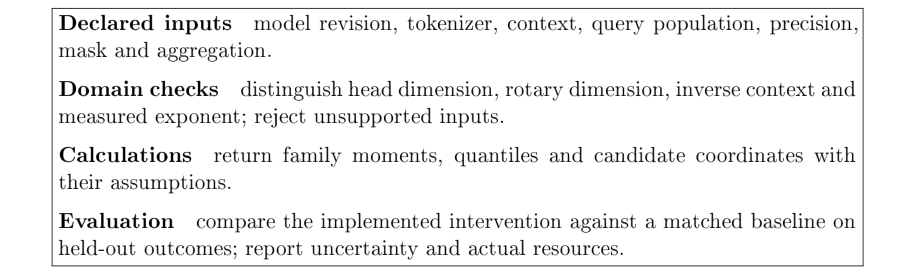
Corrected calculation and evaluation workflow. A configuration calculation does not supply a task verdict. The obsolete interface screenshot is preserved only in the predecessor archive.
21.1 Recorded endpoints and source layout
The manuscript records the following locations. Availability, authentication, licensing and current service behavior were not tested in this local review.
|
Application |
|
|
Field guide (EN/ES) |
|
|
Repository |
|
|
Mirror |
|
|
Registry |
The archived layout includes python/taf_browser.py for calculations, js/main.js for orchestration, js/i18n.js for language strings, an HTML/CSS shell and a CLI measurement script. The November 5 snapshot freezes relevant files for comparison; it is not a complete, freshly tested reconstruction of every historical release. The described architecture combines browser Python via Pyodide and optional WebGPU synthesis with remote model/configuration retrieval. Local numerical execution does not imply that identifiers or requests never leave the tab: Hub search and remote downloads require network requests. The former blanket privacy claim, automatic gated-model access claim, universal architecture coverage and perpetual zero-cost promise are withdrawn. Their verification would require the exact deployment, request paths, authentication and licenses.
Historically, the interface offered a TAF Card, comparison forms, a small language-model routing component, a CLI command builder and a phase viewer. The CLI measures profiles when supported; a browser configuration formula does not measure them. The phase viewer’s stored rows are a panel with provenance limits, not observations generated by opening the application. English, Spanish, French and Chinese strings were described in the interface record; this audit does not certify translation completeness or current keys.
21.2 The five historical recipes and their current scope
X-1: cost comparison.
A cost comparison needs explicit prices, throughput, utilization and a tested quality target. The old alpha-S gate cannot decide whether training or self-hosting will meet that target (Appendix H). No present pricing or deployment recommendation is made here.
X-2: long-context viability.
The old composition of \(\gamma _P\), \(d_{\rm inv}\) and \(2d_{\rm inv}\) returns an algebraic length. It does not predict retrieval accuracy: \(d_{\rm inv}(\theta ,\gamma _P)=T\) by construction. Configuration-only retrieval verdicts and implied optimal base multipliers are withdrawn. Section 12 retains the saved task-specific comparisons and short-context costs.
X-3: training budget.
Parameter count and token budget are resource inputs. The assumed 400M cutoff and alpha-S score do not establish induction circuits or a training go/no-go criterion. A future estimator needs measured throughput and an independently specified quality objective.
X-5: hardware estimates.
The archived GPU catalogue and price/rate outputs are historical estimates. For a homogeneous cache, its basic storage is \(2BLNH_{\rm KV}d_{\rm head}b\) bytes, with batch \(B\), layers \(L\), retained positions \(N\), KV heads \(H_{\rm KV}\) and \(b\) bytes per scalar; real layouts can add padding, scales, metadata and allocation overhead. A hypothetical window can change \(N\), but \(D_f\) does not predict throughput or a safe compression ratio. Bandwidth, kernel implementation and measured quality are separate inputs. No USD/token or tokens/second ranking is certified.
X-19: cache mass and task outcomes.
The continuous quantile and exact discrete cumulative sum quantify mass conditional on the fitted family. Neither yields a universal PPL penalty. The configuration-only strategy ranking is withdrawn; compare actual policies with an uncompressed baseline on the intended workload and record KV head counts, precision, memory and timing.
21.3 Later mode catalogue and withdrawn diagnostic rules
The historical v0.4–v0.7 description claimed 22 modes, but the displayed list has 18 named rows plus Ask, Compare and Phase diagram: 21 named modes under that convention. Recipes and modes are overlapping interface concepts. No unexplained twenty-second mode is inferred or certified by this audit.
X-21: size-dependent imprint hypothesis.
The proposed formula was \(\gamma _{\rm random}=\gamma _P+\nu \log _{10}(P/(14\, \mathrm M))\), with \(\nu =-1/(2\pi )\). A rotation period does not derive that regression slope. The reported \(p=.022\) from a selected panel does not validate the fixed coefficient or identify anomalous training. The five-axis regression also used response-derived predictors (Section 5.5). Direct profiles with matched protocols are required; an error relative to this formula cannot diagnose a conversion or fine-tuning fault.
X-22: descriptive compute/context statistic.
The old \(K=\gamma \log (N^2D)\) used \(D=20N\) rather than each model’s observed training tokens. Its value depends on the counting units; an explicitly dimensionless version would need reference counts \(N_0,D_0\). The historical \(51.2\pm 16.8\) is a panel mean and spread, not an invariant or a calibrated anomaly threshold. The example \(K=74.6\) has \((74.6-51.2)/16.8=1.392857\) standard deviations, not established statistical outlier status. It is outside the quoted rounded one-spread band \([34,68]\); those two statements are compatible but do not imply a model defect.
X-23: corpus contrasts.
The old recipe used text-minus-random, opposite to the current \(\Delta \gamma =\widehat\gamma _{\rm random}-\widehat\gamma _{\rm text}\). Neither sign detects induction heads universally. The historical subgroup means \(-.19\) and \(+.03\) cannot be transferred between conventions or used as a substitute for circuit measurements and held-out ICL tests.
|
Mode |
Intended function and necessary qualification |
|
Profile |
Collect metadata, formulas and recorded profiles; distinguish measured and predicted fields. |
|
Unmask |
Inspect position/scaling settings; configuration limits do not measure practical context quality. |
|
NIAH to Reason |
Historical retrieval/reasoning estimator; architecture-only pass rates are unvalidated. |
|
LongScore |
Present stored long-context comparisons; retain benchmark versions and protocols rather than certify current rankings. |
|
Quant |
Proposed quantization-effect estimator; architectural fields alone do not establish a gamma or PPL change. |
|
Inspect config |
Display supplied fields; missing or unsupported fields need explicit handling. |
|
Contamination |
Summarize exposure hypotheses; release dates and priors do not detect actual training contamination. |
|
Drift |
Compare evaluation metadata; a score gap alone does not identify a bug or quantify numerical noise. |
|
Arena CI |
Fit a paired-comparison model and uncertainty when raw votes and sampling assumptions permit it. |
|
Saturation |
Compare stored score ranges; apparent saturation and alternative benchmarks require dated evidence. |
|
Solutions |
Index documented evaluation issues and tools; a linked remedy is not universally applicable. |
|
Chat-template |
Identify formatting conventions and build commands; an omitted template has no universal factor-two accuracy effect. |
|
Diagnose CLI |
Generate a measurement command; actual model support and runtime dependencies must be checked. |
|
JSON CoT |
Flag output-field order; schema order alone does not prove or disprove reasoning quality. |
|
PEFT Lint |
Inspect scripts for known patterns; static checks cannot establish a successful training run. |
|
Cache Diff |
Estimate provider-specific cache effects using explicit current rules and measured hits. |
|
Spec-Decode |
Compare tokenizers; mismatch is a compatibility concern, not proof that every method is slower than baseline. |
|
Token Tax |
Count tokens with named tokenizer versions; count differences are separate from service prices and task accuracy. |
Verification layers.
The older interface described twelve runtime algebraic checks and 37 theorem badges. A numeric residual, a symbolic simplification and a proof-assistant theorem have different contracts. The equation \(2\eta ^2+\eta \gamma _\chi +1=0\) needs its own definition or constraint on \(\gamma _\chi \); it is not an identity for arbitrary independently measured quantities. Likewise \(\beta \chi =-1\) uses the specific legacy definitions in the sub-one domain. A manifest count does not certify all claims in this manuscript. The earlier 20-lemma Isabelle audit retains the scope summarized in Appendix A. This edition additionally integrates the eight verified groups in Appendix K; its complete Isabelle/HOL session audited 300 named project facts. The count includes intermediate facts and is not a count of independent empirical claims.
21.4 Formula map: calculation versus empirical interpretation
The map lists actual mathematical inputs, including a fitted exponent when needed. It is a dependency map of calculations, not an established causal chain from configuration to task performance. Object Inputs Output and scope \(\gamma _P\) \(\theta ,T{\gt}0\) Candidate in \((-1,1)\); not a measured slope. \(d_{\rm inv}\) \(\theta ,g\) Inverse coordinate for \(-1{\lt}g{\lt}1\); no information cutoff. \(2d_{\rm inv}\) \(\theta ,g\) Historical threshold proposal; no retrieval pass-rate guarantee. \(D_f\) \(g,N,f\) Mass quantile; specify continuous or discrete support. Soft decay \(w\) \(g,d_{\rm inv},d\) Multiplicative weight, or \(\log w\) score bias inside its domain; PPL requires evaluation. Base ratio \(g_{\rm target},T,\theta \) Inverse-candidate multiplier; not universal NTK optimality. Inverse base \(g_{\rm target},T\) Positive base for \(-1{\lt}g_{\rm target}{\lt}1\); task suitability unvalidated. \(\alpha _S\) \(R_c,N,D\), reference scales Historical heuristic; go/no-go interpretation withdrawn. \(n_{\rm active}\) \(d,\theta ,d_{\rm rot}\) Exact uncycled-plane count with specified pairing; no proof of semantic function. \(L_{\rm crit}\) Defined measurement protocol Historical depth hypothesis; not an architecture-only certified limit. \(C_V\) \(g,N\) Finite-family response, finite at one; no calibrated forgetting alarm. \(\chi \) \(g\ne 1\) Defined reciprocal \(1/|1-g|\); distinct from finite Fisher information. \(S_N\) \(g,N\) Shannon distance entropy; asymptotics require a specified fixed-\(g\) regime. \(\Delta \gamma \) Matched random/text fits Descriptive contrast, not a circuit or architecture classifier. \(e^{S_N}\) \(g,N\) Effective number of supported distances, not a reasoning ceiling. \(I_{\rm total}\) Stated coordinate convention Historical information-budget proposal, not derived channel capacity. Entropy-slope test Multiple supports and fits Finite-size diagnostic proposal; not a guaranteed phase classifier. \(R_{\rm patch}\) Intervention and baseline Protocol-specific recovery statistic; causal claims require controlled patching.
21.5 Application role and remaining work
A useful interface should expose provenance, mathematical domains, missing fields and uncertainty. Updating it to match these corrections is separate implementation work; the companion’s November 18 corrections are documented separately. This manuscript audit neither verifies the live service nor publishes application changes. Agreement between a displayed formula and a worked example is an arithmetic check; empirical validation requires independent observations.
Companion reading and software.
The current companion documentation connects the finite-family formulas, the Padé candidate and measured attention profiles to distinct workflows. The field-guide measurement chapter explains how to retain a query and fit protocol; the TAF Agent chapter explains the browser and CLI routes. TAF Agent’s formula contract specifies the finite support, domains and provenance of displayed values. Its November 18 software-and-guide corrections precede this November 19 manuscript edition. The links are reading and calculation routes, not independent evidence for a trained-model claim. The companion Blueprint maps statements, proofs, figures and four illustrative labs. The version DOI of this edition is 10.5281/zenodo.24379538; the older Zenodo record remains the historical edition.
22 Conclusion
Coordinate and field audit.
The preserved B3 and amplification observations describe the implemented coordinate operations; their former frequency-specific causal interpretations are withdrawn. The field null reproduces a slope near the initial checkpoint, and spectral statistics require explicit basis and aggregation conventions. These are necessary corrections to the empirical interpretation, not new trained-model results. Matched plane interventions and fixed-context controls remain necessary before any mechanistic or deployment prescription.
Instrument control precedes physical interpretation.
The uniform-causal E4 control demonstrates that the measurement can produce a high-\(R^2\) apparent power law without learned attention. This weakens the initial-panel comparison as evidence for a geometric law. The fixed-query QL control does not share that slope confound on its audited fit range. Future model comparisons must preserve query sets, supports and null conventions; synthetic controls alone do not settle how much real-model behavior remains.
Attention-distance profiles provide useful empirical descriptions when their corpus, support and measurement protocol are stated. The finite power-law family supplies exact identities for normalization, entropy, Fisher information and a formal heat capacity. Maximum entropy selects that family under a prescribed log-distance moment and reference measure. Rotary geometry alone does not establish that trained attention solves this optimization problem.
The configuration-based Padé expression remains a candidate, not a universal prediction of the measured exponent. Its withdrawn derivation cannot be restored by algebraically inverting the same expression. The mixed initial comparison with 13 recorded bases has mean absolute exponent error \(0.167766\) and median absolute relative error \(19.2144\% \). The selected-case statistic is withdrawn because its membership and calculation could not be reconstructed. In the separate October replay, 25 of 42 historical identifiers have recovered measurements, and the stored candidate has rank correlation \(-0.445\) against 19 available QL fits. Protocol changes prevent interpreting those disagreements as a controlled estimate of one architectural or instrumental effect.
Compression and context experiments remain empirical observations under their recorded conditions. A family mass quantile does not guarantee autoregressive task accuracy, and an inverse-candidate base does not determine an optimal context-extension setting. The frozen-row output-error bound is useful within its fixed-score and fixed-value assumptions. The November intervention campaign provides a separate test of effect prediction on 32 shared prompts for three models; prediction gains do not establish improved model capability.
The next empirical steps are matched-protocol estimation with sequence uncertainty, prospective comparison against alternative profile families, and controlled task evaluation of proposed interventions. Circuit, geometric, physical and hallucination interpretations need evidence beyond exponent matching. Appendix K supplies eight verified groups that sharpen the mathematical part: null calibration, finite-grid and mixture bounds, quantile order, finite-family stability, truncation, softmax and a conditional cosine-to-power approximation. These results cover their stated hypotheses; they certify neither the empirical pipeline nor scientific novelty.
This edition integrates the November 12 full-document consistency review. The rational flow and map have corrected domains; physical identifications without the required structures are withdrawn. Adaptive historical controllers fail prefix causality, the fixed-point panel is uninformative by construction, and the V1/V2 comparison uses attention temperature in the context slot. The exact displaced arguments and complete predecessors are archived; Appendix J records their replacement; obsolete arguments are preserved outside the current manuscript. Historical provenance gaps and untested empirical hypotheses remain open. The audit is not a certificate that all scientific claims are error-free.
Code and data provenance.
The archived calculations and their limitations are described in Section 8. The companion project is github.com/karlesmarin/tafagent. This edition introduces no new model inference or software deployment. It incorporates the previously verified November 19 formal developments without modifying their proof sources. The source package includes the exact verified snapshot, its build and dependency receipts, a theorem-to-source map, and the manuscript integration and build checks.
A Symbolic Checks and Formal-Proof Scope
The historical SageMath scripts record symbolic explorations, not a blanket certificate of every displayed formula or interpretation. The accepted local Isabelle session from the earlier audit contains 20 scoped lemmas with quick-and-dirty disabled and no reported oracle dependencies. Its continuous variance lemma assumes the first two moments; it does not mechanize the integral. Its limitations remain unchanged by the new appendix. The earlier prior-art audit found eight direct own-repository precedents and one PDI precedent after reparametrization; novelty was not established for any of the twenty lemmas.
The eight-group extension is now presented in Appendix K, with its complete 300-fact Isabelle/HOL session and a map to the supplied proof sources. That development is separate from the earlier 20-lemma audit.
The corrected mathematical checks are:
On continuous \([1,N]\), \(N{\gt}1\), the normalizer is \(Z_c=(N^{1-g}-1)/(1-g)\) with limit \(\log N\) at one. On discrete distances it is \(Z_N=\sum _{d=1}^N d^{-g}\) with value \(H_N\) at one.
In the finite discrete family, \(U_N=-\partial _g\log Z_N\) and \(S_N=\log Z_N+gU_N\) are exact. The latter is Shannon entropy, not an entanglement or Cardy formula.
\(I=\operatorname {Var}(\log d)\) and \(C_V=g^2I\) are finite for fixed \(N\). The value \((\log N)^2/12\) at one belongs to the continuous family.
The continuous \(f\)-quantile is \([(1-f)+fN^{1-g}]^{1/(1-g)}\) with limit \(N^f\) at one. The large-\(N\) expression \(Nf^{1/(1-g)}\) requires fixed \(g{\lt}1\); it is not uniform near one and is not the exact discrete quantile.
For \(N{\gt}1\), \(dU/dg=-I{\lt}0\) and \(dS/dg=-gI\), hence \(dS/dU=g\). The degenerate one-point family does not define this quotient.
\(T\sqrt2/(1-\gamma _P)=\theta +T/\sqrt2\) is an exact composition with the linear inverse, not a first-order approximation to the Padé inverse.
The November 12 deep audit additionally invokes callable modules from Curiosity, Excovery, Socrates and Triangulum. It records module hashes, symbolic residuals, high-precision finite-sum checks, positive and negative controls, and candidate-span detection. Several tools share SymPy; agreement is not four independent proofs. Some parsers/checkers return inconclusive results, retained in the machine-readable evidence rather than promoted to certificates. Candidate extraction is not exhaustive semantic validation.
B Audit of the Attempted Geometric Derivation
The earlier “full proof” mixed an exact softmax identity with unproved statistical assumptions and inconsistent boundary conditions. Its full text is preserved in the predecessor source and replacement log. The steps below state precisely what survives and what fails.
Step 1: rotary scores and cycle counts.
With the actual rotary subspace \(d_{\rm rot}=2m\), a rotary score contains both cosine and sine coefficients: \(\sum _i[a_i\cos (d\omega _i)+b_i\sin (d\omega _i)]\), plus any unrotated contribution and the attention scaling factor. Completing one cycle at a particular distance does not average a sinusoid to zero. For fixed \(d\), averaging random inputs does not average the phase itself. Nor do independent token IDs establish zero-mean independent projected representations after learned transformations. Constant isotropic coefficients, a positive residual cosine mean and cancellation of cycled planes all require separate evidence.
If, as an extra hypothesis, the expected score were \(b+a\widetilde n_{\rm active}(d)\) in an unclipped log-linear range, its log-distance coefficient would be
The earlier \(d_{\rm head}/(2\log \theta )\) omitted the coefficient \(a\) and equated the full head dimension to the rotary subspace. Even the correct conditional coefficient does not determine a learned exponent.
Step 2: averaging and the valid conditional theorem.
In general, \(\mathbb E[\operatorname {softmax}(s)]\ne \operatorname {softmax}(\mathbb E[s])\). Concentration of a denominator alone also does not replace \(\mathbb E[e^{s_d}]\) by \(e^{\mathbb E[s_d]}\). For example, with two logits \((X,0)\) where \(X=0\) or \(2\) equally often, the mean first softmax weight is approximately \(.690399\), whereas softmax of the mean logits gives \(.731059\). The interchange requires additional error control, not just a many-prompt average.
The valid statement is exact and conditional: if every logit on the chosen support has form \(s_d=c-g\log d\), then
This proves the consequence of a prescribed score profile. It does not derive that profile or \(g\) from a cycle-count geometry. The separate MaxEnt theorem likewise starts from a prescribed log-distance constraint.
Step 3: the rational candidate is not fixed by the old conditions.
For \(M_a(z)=(a-z)/(a+z)\), \(M_a(0)=1\) for every nonzero \(a\); this condition cannot select \(a=2\). The latter value gives \(M_2(1)=1/3\), not zero as previously claimed. Its zero occurs at \(z=2\), or \(T=\theta \sqrt2\), not \(T=\theta /\sqrt2\). At \(T=\theta \) it gives \((2-\sqrt2)/(2+\sqrt2)\simeq .171573\), not approximately one. One can obtain \(a=2\) by imposing the candidate derivative \(M_a'(0)=-1\), but that is a stipulated local condition; it still does not derive it from the measured attention process. The old error percentages on a selected “non-anomalous” subset neither repair these contradictions nor identify isotropy as the cause of all residuals. See the complete panels in Section 5.4.
Three distinct base mappings.
At a fixed positive \(T\), solving \(\gamma _P(\theta ,T)=g\) gives
The linear candidate instead has inverse \(\theta _L(g,T)=T\sqrt2/(1-g)\) for \(g{\lt}1\). Evaluating that different inverse on \(\gamma _P\) yields
The earlier Taylor expression used \(\theta (1+z)\) and was off by a factor two in its increment. No Taylor approximation is needed for the identity above. Finally the separate imposed relation \(g=\log \theta /\log b\) has inverse \(b=\exp (\log \theta /g)\) for \(g\ne 0\); it is neither of the other two inverses. At \(\theta =10000,T=1000\), the Padé inverse returns 10000 exactly and the linear composition gives 10707.106781. Their difference is \(7.071068\% \) of 10000, not a sub-\(0.5\% \) inverse error. At \(T=5000\) it is \(35.355339\% \), not below \(2\% \).
C Formula Table
The catalogue below gives the mathematical objects used in the corrected summary. The full earlier catalogue is preserved in the separate predecessor archive indexed by Appendix J. Their presence in that archive does not confer validation or novelty. The current status of all twenty original finding groups is listed in Appendix G.
Object Expression Scope Finite family \(p_\gamma (d)=d^{-\gamma }/Z_N\), \(Z_N=\sum _{d=1}^N d^{-\gamma }\) Integer \(N\ge 1\), real \(\gamma \), counting measure. Log moment \(U_N=\sum _d p_\gamma (d)\log d\) Equals \(-\partial _\gamma \log Z_N\). Entropy \(S_N=\log Z_N+\gamma U_N\) Exact finite-sum Shannon entropy; \(0\le S_N\le \log N\). Fisher metric \(I(\gamma )=\operatorname {Var}_{p_\gamma }(\log d)\) Finite at every real \(\gamma \) for fixed \(N\); evaluate directly at zero. Formal heat capacity \(C_V=\gamma ^2I(\gamma )\) Family susceptibility, not an identified task sensitivity. Intrinsic length \(\left|\int _{g_1}^{g_2}\sqrt{I(g)}\, dg\right|\) Distance along this statistical family. Continuous normalizer \(Z_c=(N^{1-\gamma }-1)/(1-\gamma )\); \(Z_c(1)=\log N\) Lebesgue measure on \([1,N]\), \(N{\gt}1\); not the discrete normalizer. Variance at one \(C_{V,c}(1)=(\log N)^2/12\) Continuous only. For discrete distances use the variance of \(\log d\). Free-energy coordinate \(-\log Z_N\) Dimensionless coordinate; division by \(\gamma \) gives the thermal convention for \(\gamma \ne 0\). Discrete mass window \(\min \{ k:\sum _{d=1}^k d^{-\gamma }\ge fZ_N\} \) Integer distance quantile; \(0{\lt}f{\lt}1\). Continuous mass window \([(1-f)+fN^{1-\gamma }]^{1/(1-\gamma )}\); \(N^f\) at \(\gamma =1\) Quantile of the continuous family, not an accuracy bound. Padé candidate \((2\theta -T\sqrt2)/(2\theta +T\sqrt2)\) \(\theta ,T{\gt}0\); range \((-1,1)\); empirical identification unestablished. Inverse base \(T\sqrt2(1+g)/(2(1-g))\) \(-1{\lt}g{\lt}1\), \(T{\gt}0\); candidate inversion, not a task optimum. Inverse context \(d_{\rm inv}=\theta \sqrt2(1-g)/(1+g)\) \(-1{\lt}g{\lt}1\), \(\theta {\gt}0\); not a validated retrieval ceiling. Shifted base \(b(T)=\theta +T/\sqrt2\) Exact coordinate definition; different from the inverse base. Log base ratio \(\log [b(D)/b(N)]\) Signed coordinate change, not established information loss. Threshold exponent \(d_{\rm eff}=1/\gamma \), \(\gamma {\gt}0\) Records a weight-threshold count exponent, not measured geometric dimension. Effective support \(\exp S_N\) Entropy effective number within the chosen family, not a task context limit. Frozen-row bound \(\| o-o_K\| \le \epsilon \, \operatorname {diam}\{ v_j\} \) Fixed scores and values, renormalized retained row, removed mass \(0\le \epsilon {\lt}1\). Soft decay \(w(d)=(1-d/d_{\rm inv})^\gamma \) inside \(0{\lt}d{\lt}d_{\rm inv}\) For positive \(\gamma ,d_{\rm inv}\): use \(\log w\) as a score bias; an empirical proposal, not a geometry theorem. Corpus contrast \(\widehat\gamma _{\rm random}-\widehat\gamma _{\rm text}\) Matched-protocol descriptive statistic; not a causal architecture identifier.
Colour: green = yes / holds.
Asymptotic entropy is a separate statement.
For fixed \(0{\lt}\gamma {\lt}1\),
At one it is \(\tfrac 12\log N+\log \log N+O(1)\); above one it converges to \(\log \zeta (\gamma )-\gamma \zeta '(\gamma )/\zeta (\gamma )\) for fixed \(\gamma {\gt}1\). These regimes cannot be merged into the former \((1-\gamma )\log N\) expression.
D Zipf and Attention: Saved-Panel Audit
For two members of the same finite power-law family with integer \(N{\gt}1\), equality of log moments identifies equal exponents on the same support and reference measure (Section 6.3). Equal moments of arbitrary distributions do not imply this conclusion. Vocabulary ranks and token distances are different observables. The saved Zipf file contains eight attempted entries: seven successful estimates and one gated-access failure for Gemma. Replaying the seven pairs gives Pearson \(r=-.505314\); this is a valid descriptive cross-row statistic, not an undefined constant-vector calculation.
|
Model |
rank exponent |
text attention exponent |
|
Pythia-70M |
.997365 |
.747602 |
|
Pythia-1B |
.997365 |
.931108 |
|
Pythia-1.4B |
.997365 |
.705073 |
|
Llama-2-7B |
1.232283 |
.287057 |
|
Mistral-7B |
1.164898 |
1.060750 |
|
Qwen2.5-7B |
1.015546 |
.996695 |
|
Llama-3-8B |
1.007281 |
1.045476 |
There are three Pythia rows, not four: 2.8B is absent from this JSON. Their rank exponents are exactly equal in the stored file, so that subgroup’s Pearson correlation is undefined, not zero or approximately \(-.5\). Their attention exponents span \(.705073\)–\(.931108\). Shared tokenization reduces independent variation in the rank statistic, but does not prove that tokenization uniquely caused the pooled negative correlation. No adjusted positive correlation is supplied. “BPE” and “SentencePiece” are not mutually exclusive tokenizer categories.
The historical JSON’s delta field uses text-minus-random, opposite to the current random-minus-text convention. The Llama-2 record retains its unresolved acquisition/quantization provenance and cannot establish a precision artifact. A controlled comparison would need matched corpora, tokenization, support, acquisition and uncertainty, with a hypothesis that actually links the two observables. Varying the base alone does not prove the equality of their exponents.
E Quick Reference Card
Purpose. Separate measurement, family calculations and intervention tests. The original configuration-only deployment card is preserved only in the separate predecessor archive indexed by Appendix J.
1. Define and measure the observable.
Record immutable model and tokenizer revisions where available, corpus snapshot, precision, attention backend, query selection, distance support, bins and aggregation. Fit the declared profile and report sequence-level uncertainty. A large \(R^2\) alone does not identify an architecture or certify a power law. Compare alternative families on the same observations and loss.
2. State which exponent is being used.
Use \(\widehat\gamma \) for a measured fit and \(\gamma \) for a family parameter. The configuration candidate \(\gamma _P=(2\theta -T\sqrt2)/(2\theta +T\sqrt2)\) lies in \((-1,1)\) for positive inputs and cannot stand in for every observed exponent. Use the explicitly identified comparison panels in Section 5.4, not the withdrawn selected-case accuracy claim. Corpus contrasts require a matched protocol and do not alone identify circuits.
3. Compute the appropriate mass window.
For integer token distances use
For the distinct continuous density on \([1,N]\), use
State \(N{\gt}1\) and \(0{\lt}f{\lt}1\). These are mass quantiles under a chosen family, not measured memory savings or guarantees about accuracy.
4. Interpret inverse Padé as algebra.
For \(-1{\lt}g{\lt}1\) and \(T{\gt}0\),
No task optimum follows. Substituting the candidate into its context inverse returns \(T\) identically and cannot independently validate a retrieval horizon. The exponential and linear legacy inverses are different functions.
5. Evaluate the intervention.
Use held-out paired examples to measure perplexity or task quality together with actual resource savings. Include the unchanged model and relevant baselines. Keep missing measurements distinct from zero outcomes. Report the scope of uncertainty and failure cases. An anomaly score suggests a hypothesis; causal circuit identification requires additional interventions.
F Productive Negative Results
Revision of 7 November 2026
The negative-result record is retained in full. Numerical results retain their original protocol and provenance limits; their preservation is not a fresh replication. A failed physical analogy does not establish a replacement physical theory. The corrected baseline and instrument distinctions apply to positive and negative outcomes alike.
The historical identifiers below are retained, including the original jump from NR-10 to NR-12; no NR-11 result is supplied. They are not nine independent replications. A failed candidate, a weak correlation and an uninformative experiment have different meanings. None establishes a replacement law or an inference-time invariance of learned attention.
NR-1: a poor beta-family parameterization.
The historical 14-model symbolic regression reports \(R^2=.052\) for the chosen geometric parameterization. This does not rule out all beta distributions or prove that power and exponential families exhaust the alternatives. MaxEnt uniqueness holds under its stated constraint; a failed regression is not an additional uniqueness proof.
NR-2: nonconstant radius/training-length ratio.
The historical 14-model coefficient of variation \(.885\) describes the selected ratios \(D_{.9}/T_{\rm train}\). It does not establish any universal replacement invariant, nor derive the empirical scatter from \(\gamma _P\).
NR-3: H3 applicability was not quantified by the proposed bound.
The legacy account mixes short/long distances 50/100 with a later assertion about distance 1000, and reports nonpositive log-probability differences for its tested RoPE models. These protocol settings cannot be reconciled from that prose alone. The continuous zero-count scale \(2\pi \theta \) is not an identified degradation threshold, and the proposed ratio \(n_{\rm dead}(d_{\rm long})/N{\gt}1.5\) has no validated applicability theorem. The observed contrasts do not establish the claimed root cause; a recoverable protocol, a nondegenerate baseline contrast and controlled patching are needed.
NR-4: Attention-entropy proxy (\(|r| \le 0.23\)).
We hypothesised that per-layer attention entropy \(H_\mathrm {attn}(\ell )\) is an inverse proxy for the H3 recovery ratio \(R(\ell )\): when the model cannot recover (\(R=0\)), attention should be uniform (\(H_\mathrm {attn} \approx \ln T\)); when recovery is complete (\(R=1\)), attention should be concentrated (\(H_\mathrm {attn} \approx 0\)). Pearson correlations across three GPT-2 variants at the critical head \(h_0\):
|
Model |
\(r(H_\mathrm {attn},\, 1-R)\) |
verdict |
|
gpt2-medium |
\(-0.15\) |
opposite direction |
|
gpt2-large |
\(-0.23\) |
opposite direction |
|
gpt2-xl |
\(+0.05\) |
expected sign, small |
The written hypothesis predicts a positive correlation with \(1-R\). Thus \(+.05\) has the expected sign, while the two negative coefficients do not. Small sample correlations do not establish statistical independence, geometric orthogonality, induction-head causation or superiority of gamma as a positional-information summary. The three numbers remain historical reports.
NR-5: Content-range slopes and their range-specific nulls.
We predicted \(\gamma _\mathrm {long} {\lt} \gamma _\mathrm {short}\) from the instantaneous formula \(\gamma = 1 - d\sqrt{2}/\theta \): longer ranges should give slower decay. Empirical power-law fits over \(d \le 100\) versus \(d \ge 200\) give the following historical rounded values, whose underlying run is not identified:
|
Model |
\(\theta \) |
\(\gamma _\mathrm {short}\) |
\(\gamma _\mathrm {long}\) |
\(\Delta \) |
|
pythia-70m |
10K |
0.661 |
0.856 |
\(+0.195\) |
|
LLaMA-3-8B |
500K |
0.812 |
1.041 |
\(+0.229\) |
|
Qwen2.5-7B |
1M |
0.904 |
0.854 |
\(-0.049\) |
Colour: blue shade = the number’s size within its column.
The displayed rounded Qwen slopes subtract to \(-.050\); the retained \(-.049\) was the historical reported difference, which cannot be recovered exactly from those rounded entries. Different fitting ranges and the variable-length null affect slopes. For the E4 grids \(\{ 30,50,100\} \) and \(\{ 200,500,1000,2000\} \), the uniform-null slopes are \(0.525737\) and \(0.913768\), giving \(\Delta _0=0.388031\). Subtracting that null contrast from the reported deltas gives approximately \(-0.193\), \(-0.159\) and \(-0.437\). Conditional on those grids, all three have the formerly predicted sign after null subtraction; “direction reversed” is therefore withdrawn. This does not validate the instantaneous candidate.
Replaying the separately identified text JSONs P10, P16 and P13 on exactly those grids gives raw contrasts \(-0.074078\), \(-0.056949\) and \(-0.047435\); their null-subtracted contrasts are \(-0.462109\), \(-0.444979\) and \(-0.435466\). These files do not reproduce the historical rounded table, so the two sets are not silently merged. No paired confidence intervals are available for either range comparison. P4 likewise requires range-specific null residuals before a curvature sign is interpreted.
NR-6/7/8 — Three inference-time perturbation records.
Three experiments attempted to manipulate \(\gamma \) at inference time:
(a) Temperature sweep (\(\tau \in [0.3, 2.0]\), pythia-70m, 4-bit weights, bf16 compute, random-token lengths \(d+200\), query \(d+199\) and key 199, matching the protocol of (b), \(N = 30\) prompts): fitting \(\gamma (\tau ) = \gamma _0\, \tau ^{-\beta }\) gives \(\beta = -0.008\), \(R^2 = 0.014\)—no monotonic trend. The replayed minimum is \(.674860\), maximum \(.757621\), and full range \(.082761\). The largest absolute change from the \(\tau =1\) baseline \(.749359\) is \(.074499\); the range is not a symmetric \(\pm .083\) interval. The eight stored means at \(\tau =1\) are exactly identical to the eight means at base 10000 in (b), not merely equal after rounding. Both scripts reset the same random generator and use the same extraction. This explains the shared baseline at the data level; without run identifiers it does not establish whether it was acquired once or twice. It is not independent replication evidence. Softmax is invariant to adding a common scalar, not to scaling logits. This recorded slope stability does not establish invariance of the attention matrix.
(b) Inference-time base sweep. The nine Pythia-70M settings use 4-bit weights with bfloat16 compute, 30 random-token prompts per distance, all heads/layers and lengths \(d+200\). The saved helper patches the actual partial-rotary inverse-frequency buffers and their original copies. No weights are retrained. All nine fits replay from the saved eight-distance means. Their range is \(.478980\)–\(.772036\) (width \(.293056\)), not \(\le .08\); the largest departure from the nominal-base fit \(.749359\) is \(.270379\). The weakest power fit has \(R^2=.610621\) at base 4000. The regression of observed on candidate slopes remains \(.152860\) with \(R^2=.144304\). The matched uniform-attention null is \(.439001\) for this \(d+200\) instrument. These observations contradict faithful candidate tracking but establish neither invariance to base changes nor a mechanism in which weights encode the training base. The complete panel is retained below.
|
\(\theta \) |
\(\gamma _P\) |
\(\widehat\gamma \) |
\(R^2\) |
|
2000 |
0.171573 |
0.714375 |
0.974191 |
|
4000 |
0.477592 |
0.478980 |
0.610621 |
|
6000 |
0.618513 |
0.539640 |
0.830007 |
|
8000 |
0.699558 |
0.744934 |
0.987758 |
|
10000 |
0.752201 |
0.749359 |
0.986877 |
|
15000 |
0.827684 |
0.753198 |
0.961704 |
|
25000 |
0.892920 |
0.772036 |
0.970149 |
|
50000 |
0.944987 |
0.705375 |
0.916144 |
|
100000 |
0.972110 |
0.700762 |
0.980592 |
Colour: blue shade = the number’s size within its column.
(c) Learned band scalars (192 trainable log-scalar parameters, Adam \(3{\times }10^{-3}\), 300 steps, targets \(\gamma \in \{ 0.5, 0.65, 0.9, 1.0\} \)): maximum \(|\Delta \gamma | = 0.063\); 5 of 6 layers converge to \(\alpha = 1.000\) exactly; perplexity remains at the random-token baseline (\(\mathrm{PPL} \approx e^{10}\)). Scaling \(QK^\top \) by \(\alpha ^2\) generally changes softmax; the reported optimization outcome requires an implementation and objective audit.
|
Perturbation |
Range |
\(|\Delta \gamma _\mathrm {obs}|\) |
Blocking mechanism |
|
Temperature \(\tau \) |
\([0.3,\, 2.0]\) |
\({\le }0.08\) |
No mechanism established |
|
\(\theta \)-steering |
\([0.2,\, 10]\times \theta _\mathrm {train}\) |
\(0.2704\) |
No mechanism established |
|
Learned scalars |
192 params, 300 steps |
\(0.063306\) |
No mechanism established |
Colour: red = no / fails.
The three protocols do not establish invariance of attention or identify a common blocking mechanism. Their estimators, optimization objectives and precision differ. The recorded failure to track a candidate is negative evidence for that candidate under the tested conditions, not confirmation that it describes an inaccessible structural exponent.
NR-9 — The spectral scaling claim depends on the instrument.
The old Pythia-1B head-dimension correction changed the reported reciprocal ratio from about \(1.38\) to \(1.111\), but did not repair full-head grouping, rotary pairing or the aggregation ambiguity. Replaying the five saved Pythia records gives a strong sample correlation \(r=-0.986580\) for the reciprocal ratio with head dimension and \(r=+0.987556\) for \(M_{\rm hist}\). These are ordinary Pearson correlations over five confounded sizes, not causal laws or partial correlations. The field-dispersion statistic has its own context-length null and missing-data rule (Section 14.3). The episode supports instrument auditing, not a claim of no architectural effect or a validated semantic score.
NR-10 — Coordinate-pruning costs do not validate a layer boundary.
Section 11.7 preserves the v1 and complete v2 records, their evaluation settings and the exact regression conventions. The available script’s selected high-index output coordinates are outside the rotary subspace in the audited Pythia-1B and 2.8B configurations. The observation is therefore a coordinate ablation, not established removal of alive RoPE bands. For a selected data set \(S\), the descriptive model is
The original common coefficient \(0.175\pm 0.005\) and \(r{\gt}0.99\) claims are withdrawn. The v2 positive-point slopes are \(0.189964\) (1B, three points) and \(0.313581\) (2.8B, four points); through-origin slopes are \(0.153883\) and \(0.167242\). The two-point 1B v1 fit is another subset. Small positive cost at one layer does not establish a harmless pruning boundary; increasing the intervention produces larger recorded costs. It also does not turn an entropy identity into a pruning prescription.
NR-12 — The three-model soft-decay comparison has no validated boundary.
The full four-policy table is in Section 11.6. Baseline has the smallest recorded PPL for 2.8B, soft decay for 1.4B and hard \(D_f\) for 1B. The former proposed rule is retained only as an unvalidated hypothesis:
The 2.8B improvement relative to hard-cutoff PPL is \(1.155\% \); \(20.729\% \) uses the excess over baseline as denominator. Hard truncation at precisely \(T_{\rm train}\) was not tested in this panel, nor were equal retained mass or a causal smoothness mechanism established. The no-op and failed cases remain part of the record. Per-chunk outcomes are needed for paired uncertainty.
NR-13: the V1/V2 comparison has a context-input error.
The saved twenty-row comparison defines \(g_{V2}=g_{V1}(1-\log 2/d_{\rm head})\). Recomputing its relative-error columns reproduces mean errors \(30.112029\% \to 29.780277\% \), median errors \(15.463669\% \to 15.997564\% \), and 13/20 row wins for V2. Thus mean error improves slightly while median error worsens; “no MAE improvement” was incorrect. The Pythia-only \(d_{\rm head}\le 80\) subset contains six rows, not four.
More fundamentally, all stored V1 values reproduce the rational formula when its context slot is filled by the corresponding master record’s T_attn, to numerical precision. That field is the rounded attention-temperature coordinate near \(1/g_{\rm obs}\), not an evaluation context length. For example, Pythia-1B uses \(T=1.0740\), yielding \(g_{V1}=.999848125\), instead of a token context such as 2000. This both confuses observables and feeds a response-derived coordinate into the prediction. The generator of this validation file was not reconstructed, but the exact stored-value match identifies the input mismatch independently. The frozen twenty rows and master record are included in the audit package.
Consequently this panel cannot validate or reject a finite-head correction at the intended contexts, establish residual causes, or make V1 canonical. The alleged continuum derivation is already withdrawn (Appendix B). A new comparison needs actual context inputs, valid rotary dimensions, prespecified fitting populations and an independent outcome; the old five-axis response-leaking fit supplies none.
Correct context-input interface and illustrative recalculation.
The replacement calculator accepts a named positive integer context_tokens, a positive base and an explicit definition of that context. It does not accept the old T_attn schema or infer context from a measured exponent. At base 10000 and head dimension 256, it gives:
|
Declared context |
rational V1 |
proposed finite-head V2 |
|
512 |
0.930122115 |
0.927603711 |
|
1024 |
0.864962305 |
0.862620328 |
|
2000 |
0.752201314 |
0.750164649 |
|
4096 |
0.550831282 |
0.549339848 |
Colour: blue shade = the number’s size within its column.
These are conditional arithmetic examples, not new measurements or a repaired twenty-model validation. The old E4 protocols use varying sequence lengths; no single context can be inferred from their aggregate slopes. A scientific comparison must declare its context convention independently and align the observation protocol. The proposed V2 multiplier still needs empirical justification. Input validation prevents the specific schema/units error; it cannot certify the scientific provenance of a user-supplied integer.
G Compendium of Critical Findings
The twenty original identifiers are retained to make the evidence traceable. This table states their current scope rather than reproducing the old novelty stars as certification. Historical numerical panels remain explicitly identified in the cited sections; the complete old compendium is stored in the separate predecessor archive indexed by Appendix J. No novelty claim is established by a symbolic identity or a formal proof alone.
ID Original topic Current conclusion Location F1 Padé predictor Algebraic candidate. Universal derivation withdrawn; initial and October panels have different protocols and denominators. §5.3 F2 Rotary geometry Exact cycle counts require the actual rotary subspace and pairing convention. Completing a cycle does not prove loss of information. §4.2 F3 Boundary at one Infinite-support summability boundary. Finite sums are analytic; \((\log N)^2/12\) is the continuous variance, not the discrete value. §7 F4 Entropy law Finite entropy bound and distinct fixed-exponent asymptotics. The old leading factor \((1-\gamma )\) is incorrect. §7.4 F5 Semantic reservoir Unsupported by the inspected masks: B3 removes unequal coordinate sets; the amplification script also changes V. §13 F6 Band dissociation Full B3 sweep retained. The larger coordinate mask has higher PPL in all six windows; no semantic/positional double dissociation. §7.4 F7 KV window Exact discrete and continuous mass quantiles are different. Recorded truncation trials do not establish a universal accuracy-preserving range. §11 F8 NTK scaling Base multiplier differs from context factor. B1 ratios hid short-context PPL costs; candidate-ranking counts do not establish Pareto dominance or a universal optimum. §12 F9 Base design Corrected table generated from the inverse equation. At \(T=4096\), targets \(0.5\) and \(0.85\) give about 8689 and 35721; task assignments are unvalidated. §12.1 F10 GQA pressure Architectural association hypothesis. Mixed configurations and corpora do not isolate a causal effect of the number of KV heads. §8.4 F11 Boiling criterion Thresholds for forgetting or loss spikes are unvalidated. A family heat capacity is not a measured risk probability. §7.2 F12 Induction threshold A universal sign transition near 400M parameters is unsupported; fitting supports and alternative mechanisms matter. §8.4 F13 SWA confinement Masking affects available keys, but the reported cross-model contrasts do not identify a universal exponent shift. §16 F14 Alignment shifts Historical base/instruction pairs retain their measured differences. They do not isolate RLHF from SFT, DPO or other changes. §15 F15 Holography A Shannon entropy bound does not establish entanglement geometry, a Ryu–Takayanagi identification or universal central charge. §7.4 F16 Fisher identity \(C_V=\gamma ^2I\) is exact in the finite family. Division by \(\gamma ^2\) excludes zero, and extrema need not coincide. §7.3 F17 RG flow The rational-coordinate differential equation and its solution are conditional algebra, not a measured training trajectory. §20.2 F18 Controller recovery Adaptive historical hooks pool future positions and fail prefix causality; their scores do not certify causal PPL. Recovery denominators differ and the Fisher prediction is withdrawn. November tests are separate evidence. §19.2 F19 Soft decay Recorded policy comparisons remain protocol-specific. The score bias is \(\log w(d)\), not \(w(d)\); no general PPL improvement follows. §11.6 F20 Pruning cost Slopes on two model experiments are descriptive fits, not a universal cost law or a cross-model uncertainty interval. The proposed layer cutoff was withdrawn. App. F
H The Historical Alpha-S Gate: Definition and Failure
This appendix defines the proposed score and recalculates all four examples from their declared inputs. The original table remains in the separate archive. Its semantic-ignition interpretation and pre-training go/no-go rules are withdrawn. The scale \(N_0=4\times 10^8\) is an assumption, not an induction-head threshold from olsson2022induction; their evidence includes two-layer attention-only models. The symbol \(N_{\rm IH}\) in the historical equations below denotes that assumed reference only.
H.1 Retained definition
where the two factors are:
The coefficient 3, centre 1.68 and token scale \(2\times 10^{11}\) were heuristic choices. The logarithmic factor is not a derivation of compute-optimal training or a probability of circuit formation; it can be negative below its chosen product reference. No Hagedorn susceptibility appears in the actual definition. The factorization does not establish a Chinchilla–Hagedorn unification.
H.2 Arithmetic on the declared historical inputs
The following table uses the displayed \(R_c\) and logarithmic-factor values as stipulated inputs. It recomputes both the gate and their product directly; the original rounded products and circuit labels are stored in the separate predecessor archive. Missing per-model token budgets are not reconstructed.
|
Model |
\(R_c\) |
stipulated \(F_{\rm Chin}\) |
recalculated \(F_{R_c}\) |
product |
|
Yi-6B |
1.28 |
5.43 |
0.083173 |
0.451628 |
|
Llama-3.2-3B |
1.33 |
5.89 |
0.109097 |
0.642580 |
|
Qwen2.5-3B |
2.03 |
6.54 |
0.890903 |
5.826507 |
|
Qwen2.5-1.5B |
3.09 |
5.85 |
0.999788 |
5.848761 |
Colour: blue shade = the number’s size within its column.
The score is not a probability and these inputs are not a validation set. Corpus-contrast signs do not supply direct circuit labels. Consequently no classification-accuracy claim or training-budget recommendation is assigned to these four arithmetic examples.
H.3 Why the design rule is withdrawn
The nine-model ratio audit in Section 16.4 supplies counterexamples to the proposed monotone gate. Its range-hull intersection is \([0.924358,3.085057]\), not a calibrated uncertainty region. The formerly cited Pythia-2.8B “observed post-IH” failure also mixes protocols: the round-3 summary has positive contrast \(+0.041\), whereas another corpus comparison has a different sign. Neither establishes a unique induction label.
The proposed alternative \(\alpha _S^{\rm v2}=F_{\rm Chin} [1+c\tanh (3(R_c-R_c^\star ))]\) was a new hypothesis, not a validated repair. Retuning a score after observing failures requires separate evaluation on held-out data with direct outcomes. No architecture, budget or training decision should use either gate as evidence that induction or retrieval will emerge.
I Bilingual Glossary
These terms refer to the specified statistical family unless an empirical measurement is explicitly stated. They do not identify a physical equilibrium or a task-level property of a trained model.
|
Term |
Definition or scope |
Spanish |
|
Exponent \(\gamma \) |
Parameter in \(p_\gamma (d)\propto d^{-\gamma }\); distinguish from a fitted \(\widehat\gamma \). |
Exponente |
|
Temperature coordinate |
\(1/\gamma \), defined for \(\gamma \ne 0\); distinct from token-sampling temperature. |
Coordenada de temperatura |
|
Normalizer \(Z_N\) |
\(\sum _{d=1}^N d^{-\gamma }\); not the normalizer of an arbitrary attention row. |
Función de partición |
|
Free-energy coordinates |
\(\Phi =-\log Z_N\); \(F=\Phi /\gamma \) for \(\gamma \ne 0\). |
Coordenadas de energía libre |
|
Log moment \(U_N\) |
\(\mathbb E_{p_\gamma }[\log d]\). |
Momento logarítmico |
|
Entropy \(S_N\) |
Shannon entropy of the declared distance distribution. |
Entropía de distancias |
|
Fisher information \(I\) |
\(\operatorname {Var}_{p_\gamma }(\log d)\) on fixed support. |
Información de Fisher |
|
Formal heat capacity \(C_V\) |
\(\gamma ^2 I\); distinct from the legacy reciprocal \(1/|1-\gamma |\). |
Capacidad calorífica formal |
|
Legacy reciprocal \(\chi \) |
\(1/|1-\gamma |\), for \(\gamma \ne 1\); not the finite-family Fisher information. |
Recíproco propuesto |
|
Summability boundary |
\(\gamma =1\) for infinite support; finite sums remain analytic. |
Frontera de sumabilidad |
|
Head dimension \(d_{\rm head}\) |
Number of coordinates in a query/key head; \(d_{\rm rot}\le d_{\rm head}\). |
Dimensión de cabeza |
|
Inverse context \(d_{\rm inv}\) |
\(\theta \sqrt2(1-g)/(1+g)\) for \(\theta {\gt}0,-1{\lt}g{\lt}1\); a candidate coordinate. |
Contexto inverso |
|
Context \(T\) |
Declared token length or comparison coordinate; never inferred from \(T_{\rm attn}=1/\gamma \). |
Contexto declarado |
|
Retained-mass window |
A quantile on a specified continuous or discrete support. |
Ventana de masa retenida |
Colour: green = yes / holds.
Acknowledgements
We acknowledge the authors of the cited research, model and dataset contributors, and the maintainers of the scientific software used in the archived work. The correction package records the local modules from Curiosity, Excovery, Socrates Audit and Triangulum, together with their source hashes and dependencies. Their symbolic and numerical checks have the scope stated in Appendix A; shared backends are not independent proofs. Responsibility for this manuscript’s definitions, interpretations and remaining empirical hypotheses rests with its author.
J Correction Register and Separate Historical Archive
This appendix replaces the earlier thirty-page reproduction of superseded arguments. The complete predecessor PDF, its source and evidence ZIP are included unchanged in the correction package. Exact displaced source is also recorded in the change log. The present manuscript contains the corrected statements; obsolete recipes and inconsistent numerical examples are not presented as an alternative current result.
ID Issue Resolution in this edition 1 Geometric prediction of trained attention Score decomposition retained; missing statistical premises made explicit. Configuration-only universality and the invalid derivation are withdrawn. Sections 5.2–5.4. 2 Variable-length measurement confound The E4 and field nulls use their actual protocols. Fixed-query QL is distinguished, with provenance and missing observations stated. Sections 9.1 and 14.3. 3 Finite and continuous thermodynamics Separate normalizers, moments, Fisher information and quantiles; correct domains and finite value at one. Sections 6.4–7.4. 4 KV performance guarantees Exact mass budgets and frozen-row bounds replace configuration-only accuracy claims; experimental policies and denominators remain distinct. Section 11. 5 Rotary/semantic band interpretation Actual rotary subspace, pairing and adjacent-coordinate masks are reported. Coordinate ablations no longer identify semantic frequency bands. Sections 11.7 and 13. 6 Inverse base and NIAH guarantees Correct inverse and explicit test protocols; algebraic identities are not independent retrieval predictions. Section 12. 7 Corpus, lexical and architecture labels Matched observables and missing query/count records are stated. Signs do not identify induction heads, SWA or GQA. Sections 14.3–16. 8 Control uses future positions New per-query reference passes prefix and partition checks. Defective historical scores are not relabelled as causal PPL. Section 19.3. 9 Wrong head-projection boundary New reference acts before the inspected NeoX mixing projection, with declared layout checks. Post-projection blocks are not called heads. Section 19.3. 10 Non-unit, incorrectly paired rotations New tables use unique frequencies and explicit pairing; norm, inverse rotation and unrotated-tail checks pass. Section 19.3. 11 Controller summaries and denominators All saved rows retained; recovery denominators and layer comparisons corrected. No Fisher-based efficacy claim. Section 19.2. 12 Potential, stability and finite-time claim Correct potential and exact trajectory; positive endpoint repels and negative endpoint attracts in the stated direction. Section 20.2. 13 Möbius domain and fixed-point test Right-half-plane mapping and determinant corrected; 0/23 clustering is structurally uninformative. Section 20.3. 14 Fractional/CFT/BTZ identifications Correct algebra and domain conditions; unsupported physical equivalences withdrawn. Section 20. 15 Complete-proof and Taylor claims Invalid averaging and normalization steps removed; inverse compositions and numerical errors corrected. Appendix B. 16 Zipf, grokking, signs and ranges Complete saved panels, proper correlation domains and actual probe support replace the earlier summaries. Appendices D and F. 17 V1/V2 context-input mismatch Old panel rejected as validation; replacement interface requires an independently declared token context. Explicit illustrative calculations are provided in Appendix F. 18 Catalogue, software and glossary Correct counts, calculation domains and terminology; obsolete verdict screenshot replaced by an evaluation workflow. Section 21 and Appendix I. 19 Alpha-S products and circuit labels Products recomputed from declared inputs. Classification marks and unsupported training-budget decisions removed. Appendix H. 20 Bibliographic errors Incorrect locators, titles and authors corrected; blogs identified; version-sensitive citation pinned; argumentative notes removed. Source metadata and exact changes are archived. 21 Contradictory archival prose and notation Erroneous prose moved to the separate predecessor archive. \(d_{\rm head}\) and \(d_{\rm inv}\) now denote distinct objects throughout.
Colour: blue shade = the number’s size within its column.
🛡️ Evidence & scope
No correction can reconstruct unrecorded observations or immutable runtime revisions. Missing D3 and October records, lexical query populations and historical model/environment revisions remain explicit provenance gaps. Claims requiring them are not asserted. New causal interventions, V1/V2 comparisons, retrieval nulls or task-quality guarantees need newly specified experiments before they can become empirical conclusions. This distinction does not leave a known erroneous formula as a current result; it prevents missing evidence from being replaced by an invented result.
K Eight Formally Verified Result Groups
This appendix integrates the eight groups of the November 19 technical note into the manuscript. Each statement below has explicit hypotheses and a readable proof; the accompanying Isabelle/HOL sources supply the machine-checked derivations. The complete session audited 300 named facts from the project’s theories. This is a count of intermediate and final facts, not 300 independent theorems. The eight auxiliary Lean lemmas have a narrower scope. The results establish mathematical implications, not that a trained model satisfies their premises. No new model measurements are introduced.
Conventions.
All logarithms are natural. Probability supports are finite and nonempty unless a continuous integral is explicitly displayed. We use \(\operatorname {TV}(p,q)=\frac12\sum _j|p_j-q_j|\) and the usual extended-real KL divergence, with zero-mass terms omitted and a positive mass divided by zero giving \(+\infty \). The real exponent \(g\) denotes the same family parameter as \(\gamma \) elsewhere; it is distinct from an observed regression slope. For finite values \(v_j\) in a real normed vector space, \(\operatorname {diam}\{ v_j\} =\max _{i,j}\| v_i-v_j\| \).
Group Result Main-text connection 1 General probe null; exact subtraction of log-slopes; fixed-query and diagonal controls Section 9 2 Strict bounds, monotonicity and limits for affine exposure Section 9.1 3 Local slope, curvature and regression bounds for positive mixtures Section 10 4 Discrete quantile order in exponent and support size Section 11 5 Smooth finite-family calculus, entropy, KL and TV bounds Sections 6.4–7.3 6 Exact truncation error, TV, KL and sharp output bounds Section 11.2 7 Sharp softmax stability and the logarithmic-score bridge Section 5.2 8 Cosine integral, explicit RoPE remainder and conditional row approximation Section 5.2
Colour: blue shade = the number’s size within its column.
K.1 Group 1: the instrument null and logarithmic calibration
Fix distances \(d_k{\gt}0\), \(x_k=\log d_k\), positive regression weights \(w_k\) with \(\sum _k w_k=1\), and \(V_x=\operatorname {Var}_w(x){\gt}0\). For any positive profile \(A\), including a fitted intercept, define
The points and weights are held fixed when two slopes are compared.
At distance \(d_k\), a probe averages allowed attention entries using weights \(\alpha _{kr}\ge 0\), \(\sum _r\alpha _{kr}=1\). If row \(r\) has \(n_{kr}\ge 1\) allowed keys, its uniform-attention null is
For every positive profile on the same grid and regression weights,
A constant null has zero slope. Keeping the same queries, support sizes and averaging weights at each distance is sufficient for a constant null.
Isabelle · ours · partshow
Only a part is in Isabelle: Requiere pesos de sonda fijos y una probabilidad finita; no caracteriza el aprendizaje.
fixed_probe_null · Isabelle/TransformerAttentionPartI/TAF_Probe.thy, line 22 — nulo uniforme de una sonda fija
lemma fixed_probe_null:
  assumes a: "\<And>k r. k\<in>K \<Longrightarrow> r\<in>R \<Longrightarrow> a k r = b r"
    and n: "\<And>k r. k\<in>K \<Longrightarrow> r\<in>R \<Longrightarrow> n k r = m r"
    and k: "k\<in>K"
  shows "probe_null R a n k = (\<Sum>r\<in>R. b r / real (m r))"
slope_covariance · Isabelle/TransformerAttentionPartI/TAF_Probe.thy, line 85 — pendiente logarítmica como covarianza ponderada
lemma slope_covariance:
  "log_slope S p x A = -fw_cov S p x (\<lambda>i. ln (A i)) / fw_var S p x"
log_slope_ratio · Isabelle/TransformerAttentionPartI/TAF_Probe.thy, line 29 — calibración con un perfil de referencia
lemma log_slope_ratio:
  assumes pos: "\<And>i. i\<in>S \<Longrightarrow> 0 < A i"
    and pos0: "\<And>i. i\<in>S \<Longrightarrow> 0 < A0 i"
  shows "log_slope S w x (\<lambda>i. A i/A0 i) =
      log_slope S w x A - log_slope S w x A0"
Trust base: 🔒 kernel only — only part of the statement is formal (see the box). Isabelle: 3 results, no oracles
Cite: Definition 7.3, p. 33, doi:10.5281/zenodo.24379538
🆕 Classical and new: Aplicación al protocolo de medición; las identidades elementales no se presentan como novedades.
↳ Used in: Theorem K.2, Theorem K.3
An allowed entry in a uniform row equals \(1/n_{kr}\). Averaging gives the displayed null, which is positive. Substitute \(\log (A_k/A_{0,k})=\log A_k-\log A_{0,k}\) in Equation (87); covariance is linear in its second argument. The covariance with a constant is zero.
En palabras.
La pendiente medida depende de la sonda y de los pesos de la regresión. Una fila uniforme puede producir un perfil aparente; restar la pendiente de un nulo construido con el mismo instrumento cancela esa contribución de forma algebraica. La prueba no describe cómo se comporta un modelo entrenado.
Fixed queries and complete diagonals.
For a fixed causal context \(T\), zero-based query indices \(i\in Q\) and fixed weights \(\alpha _i\), suppose every fitted distance is eligible for every query. Then \(A_{0,\mathrm{QL}}(d)=\sum _{i\in Q}\alpha _i/(i+1)\) is constant. By contrast, averaging every entry of the causal diagonal gives
This null strictly decreases between successive eligible distances: removing the largest member of the strictly decreasing sequence \(1/(d+1),\ldots ,1/T\) decreases its mean. Thus its OLS exponent is positive on any grid with at least two distinct distances and positive weights. The pairwise covariance identity in Group 2 proves the strict sign.
Scope and counterexamples.
The subtraction is a slope relative to a declared null, not a proof of unbiased estimation or causal attribution. Binning, exclusions and weights must be reproduced in the control; averaging and logarithms do not commute. Fixed queries are sufficient, not necessary: a row with six allowed keys and an equal-weight average of rows with four and twelve allowed keys both give \(1/6\). Also, zero covariance on a grid need not imply a constant profile. For dot-product attention without a key-dependent additive bias, setting the query projection to zero leaves every rotary query zero and gives a uniform softmax. A fixed-query probe then has zero exponent for any RoPE base. This refutes a nonzero geometry-only law over all possible weights; it does not characterize a specified training procedure.
K.2 Group 2: finite-grid bounds for affine exposure
The secant identity.
For the weights above and real observations \(y_k\),
Expanding the corresponding half-sum over all ordered pairs proves both identities. Hence the regression slope is a convex combination of secants over pairs with distinct \(x\) values, with weights \(w_iw_j(x_j-x_i)^2/V_x\).
For \(A_0(d)=c/(ad+b)\) with \(a,b,c{\gt}0\), on the nondegenerate grid of Group 1,
With the grid and weights fixed, this slope strictly decreases with \(b\). Replacing all distances by \(\lambda d_k\), \(\lambda {\gt}0\), makes the slope strictly increase with \(\lambda \); its limits as \(\lambda \downarrow 0\) and \(\lambda \to \infty \) are respectively zero and one. The amplitude \(c\) has no effect.
Isabelle · ours · partshow
Only a part is in Isabelle: Describe el sesgo del instrumento bajo exposición afín; no un mecanismo del transformer.
affine_regression_strict_bounds · Isabelle/TransformerAttentionPartI/TAF_Affine_Bounds.thy, line 83 — límites estrictos de la pendiente en una malla finita
lemma affine_regression_strict_bounds:
  assumes var: "0<fw_var S p x" and a: "0<a" and b: "0<b"
    and range: "\<And>i. i\<in>S \<Longrightarrow> l\<le>x i" "\<And>i. i\<in>S \<Longrightarrow> x i\<le>u"
  shows "a*exp l/(a*exp l+b)<fw_cov S p x (\<lambda>i. affine_log a b (x i))/fw_var S p x"
    "fw_cov S p x (\<lambda>i. affine_log a b (x i))/fw_var S p x<a*exp u/(a*exp u+b)"
affine_slope_limits · Isabelle/TransformerAttentionPartI/TAF_Affine_Limits.thy, line 99 — límites al variar la escala
lemma affine_slope_limits:
  assumes var: "0<fw_var S p x" and a: "0<a" and b: "0<b"
    and range: "\<And>i. i\<in>S \<Longrightarrow> l\<le>x i" "\<And>i. i\<in>S \<Longrightarrow> x i\<le>u"
  shows "((\<lambda>r. affine_slope S p x a b r) \<longlongrightarrow> 0) (at_right 0)"
    "((\<lambda>r. affine_slope S p x a b r) \<longlongrightarrow> 1) at_top"
Trust base: 🔒 kernel only — only part of the statement is formal (see the box). Isabelle: 2 results, no oracles
Proof: in this note·Formalized: Isabelle/HOL, by the author (public formalizations repository)·Covers: part: Describe el sesgo del instrumento bajo exposición afín; no un mecanismo del transformer.·Cite: doi:10.5281/zenodo.24379538
↳ Not used by another result of the paper.
The slope is the regression of \(f(x)=\log (ae^x+b)\) on \(x\). Its derivative \(ae^x/(ae^x+b)\) strictly increases. The mean-value theorem places each nontrivial secant strictly between the endpoint derivatives; the convex combination proves the bounds. Differentiating the finite covariance gives
The signs follow from the pairwise identity and strict opposite or common ordering. Adding \(\log \lambda \) to every \(x_k\) changes neither centered coordinates nor variance. On a finite grid, the log-profile tends to a constant at zero scale, while \(\log (a\lambda d+b)=\log (a\lambda )+\log d+o(1)\) at infinite scale. Constants disappear from the covariance, including \(\log c\).
En palabras.
Si el número de posiciones expuestas tiene la forma \(ad+b\), la elasticidad local es una fracción entre cero y uno. La pendiente OLS queda entre los valores extremos de esa elasticidad en la rejilla. Cambiar la rejilla o el desplazamiento cambia la lectura del instrumento.
For the initial E4 null, \(a=1,b=50\). Its scale-dependent slope is therefore present without learning. The boundary cases, outside the strict hypotheses, give slope one for \(b=0,a{\gt}0\), and zero for \(a=0,b{\gt}0\).
K.3 Group 3: mixing profiles changes slope and curvature
Let \(J\ge 1\), \(a_j{\gt}0\), \(g_j\in \mathbb R\), and \(A(d)=\sum _{j=1}^{J}a_jd^{-g_j}\) for \(d{\gt}0\), with coefficients and exponents independent of distance. For \(x=\log d\), put \(\pi _j(x)=a_je^{-g_jx}/\sum _\ell a_\ell e^{-g_\ell x}\). Then
The finite-grid exponent satisfies
If two component exponents differ, the local slope strictly decreases, and the mixture cannot be an exact power on any open interval.
Isabelle · oursshow
strict_mean_decrease · Isabelle/TransformerAttentionPartI/TAF_Mixture_Entropy.thy, line 38 — disminución de la pendiente local si difieren los exponentes
lemma strict_mean_decrease:
  assumes i: "i\<in>S" and j: "j\<in>S" and diff: "E i\<noteq>E j" and uv: "u<v"
  shows "emean v < emean u"
mixture_regression_bounds · Isabelle/TransformerAttentionPartI/TAF_Regression_Calculus.thy, line 65 — cotas de la regresión finita
lemma mixture_regression_bounds:
  assumes p: "finite_probability I w" and var: "0<fw_var I w x"
    and range: "\<And>i. i\<in>I \<Longrightarrow> l\<le>x i" "\<And>i. i\<in>I \<Longrightarrow> x i\<le>u"
  shows "emean u\<le>log_slope I w x (\<lambda>i. mom 0 (x i))"
    "log_slope I w x (\<lambda>i. mom 0 (x i))\<le>emean l"
non_affine_log_partition · Isabelle/TransformerAttentionPartI/TAF_Strict_Family.thy, line 38 — no afinidad de la partición no degenerada
lemma non_affine_log_partition:
  assumes i: "i\<in>S" and j: "j\<in>S" and diff: "E i\<noteq>E j" and ab: "l<u"
  shows "\<not> (\<forall>x\<in>{l<..<u}. ln (mom 0 x)=c-k*x)"
Trust base: 🔒 kernel only. Isabelle: 3 results, no oracles
Proof: in this note·Formalized: Isabelle/HOL, by the author (public formalizations repository)·Covers: the whole statement·Cite: doi:10.5281/zenodo.24379538
↳ Not used by another result of the paper.
Logarithmic differentiation yields the weighted mean. Since \(\pi _j'=\pi _j(-g_j+\sum _\ell \pi _\ell g_\ell )\), differentiating it yields the negative variance. Every \(\pi _j\) is positive, so that variance vanishes exactly when all component exponents agree. Applying the secant identity to \(-\log A(e^x)\) bounds the regression by its extreme derivatives. An exact power would have constant local slope.
En palabras.
Al sumar dos perfiles de potencia, el logaritmo de la suma suele curvarse. La derivada de su pendiente local es menos una varianza; por ello una mezcla con exponentes distintos puede aparentar un exponente dependiente de la distancia sin que cada componente cambie de ley.
Constant finite normalizers can be absorbed in \(a_j\). Changing the heads, their weights or their supports with distance can violate the hypotheses. This log-sum-exp identity does not establish that individual heads are powers or identify their computational roles.
K.4 Group 4: ordering discrete mass quantiles
Let \(N\ge 2\) be an integer and \(p_g(d)=d^{-g}/Z_N(g)\) on \(\{ 1,\ldots ,N\} \), with \(g\in \mathbb R\). For \(1\le k{\lt}N\), the prefix mass \(F_g(k)=\sum _{d\le k}p_g(d)\) is strictly increasing in \(g\). For \(0{\lt}f{\lt}1\), the well-defined integer quantile
is nonincreasing in \(g\) and, for fixed \(g,f\), nondecreasing in \(N\). These conclusions include negative exponents, zero and one.
Isabelle · ours · partshow
Only a part is in Isabelle: El mínimo que define el cuantil se usa en conjuntos finitos no vacíos.
quantile_nonincreasing · Isabelle/TransformerAttentionPartI/TAF_Power_Family.thy, line 53 — orden de cuantiles al variar el exponente
lemma quantile_nonincreasing:
  assumes fract: "fract\<le>1" and gh: "g\<le>h"
  shows "quantile h fract\<le>quantile g fract"
quantile_support_order · Isabelle/TransformerAttentionPartI/TAF_Power_Support.thy, line 8 — orden al ampliar el soporte
lemma quantile_support_order:
  assumes N: "1\<le>N" and NM: "N\<le>M" and fn: "fract\<le>F N" and gm: "fract\<le>G M"
    and order: "\<And>k. k\<in>{1..N} \<Longrightarrow> G k\<le>F k"
  shows "finite_quantile N F fract\<le>finite_quantile M G fract"
Trust base: 🔒 kernel only — only part of the statement is formal (see the box). Isabelle: 2 results, no oracles
Proof: in this note·Formalized: Isabelle/HOL, by the author (public formalizations repository)·Covers: part: El mínimo que define el cuantil se usa en conjuntos finitos no vacíos.·Cite: doi:10.5281/zenodo.24379538
↳ Not used by another result of the paper.
The defining set is finite and contains \(N\). Put \(X=\log d\) and \(L_k=\{ 1,\ldots ,k\} \). Differentiating the finite sums gives
Both groups have positive mass and every logarithm in the second exceeds every logarithm in the first. Increasing \(g\) can only advance the first crossing of \(f\). Increasing \(N\) leaves an old prefix numerator unchanged and increases its denominator; it cannot produce an earlier crossing.
En palabras.
Con soporte fijo, aumentar el exponente desplaza masa hacia las distancias cortas, así que el cuantil no puede aumentar. Ampliar el soporte puede moverlo en el sentido opuesto. Son órdenes finitos bajo las condiciones escritas, no una receta automática para elegir una ventana KV.
The integer quantile is a step function, so its monotonicity need not be strict. This family property supplies a mass budget, not a KV task guarantee.
K.5 Group 5: finite-family calculus and sensitivity
For integer \(N\ge 1\) and real \(g,h\), let \(\psi (g)=\log Z_N(g)\), \(U(g)={\mathbb {E}}_{p_g}\log d\), \(I(g)=\operatorname {Var}_{p_g}(\log d)\) and \(S(g)=-\sum _dp_g(d)\log p_g(d)\). All these functions are smooth to every order for finite \(g\), and
Writing \(L=\log N\),
Moreover,
For \(N\ge 2\), \(I(g){\gt}0\), and \(S\) has its unique maximum at \(g=0\).
Isabelle · oursshow
mean_derivative · Isabelle/TransformerAttentionPartI/TAF_Exponential_Family.thy, line 89 — derivada de la media igual a menos la varianza
lemma mean_derivative:
  "(emean has_real_derivative (-evar t)) (at t)"
entropy_derivative · Isabelle/TransformerAttentionPartI/TAF_Mixture_Entropy.thy, line 106 — derivada de la entropía
lemma entropy_derivative:
  "(canonical_entropy has_real_derivative (-t*evar t)) (at t)"
kl_integral_remainder · Isabelle/TransformerAttentionPartI/TAF_KL_Remainder.thy, line 11 — resto integral exacto de KL
lemma kl_integral_remainder:
  "finite_kl S (ep g) (ep h) = ereal ((h-g)^2 *
    integral {0..1} (\<lambda>t. (1-t)*evar (g+t*(h-g))))"
Trust base: 🔒 kernel only. Isabelle: 3 results, no oracles
Proof: in this note·Formalized: Isabelle/HOL, by the author (public formalizations repository)·Covers: the whole statement·Cite: doi:10.5281/zenodo.24379538
🆕 Classical and new: Identidades clásicas de familias exponenciales finitas, aplicadas aquí a perfiles de atención.
↳ Not used by another result of the paper.
Differentiate the finite sums using \(p_g'=-p_g(\log d-U)\). Positivity of \(Z_N\) makes its logarithm and all quotients smooth. For \(X\in [0,L]\), \({\mathbb {E}}[X(L-X)]\ge 0\) yields \(\operatorname {Var}X\le L{\mathbb {E}}X-({\mathbb {E}}X)^2\le L^2/4\). The log-ratio of probabilities gives the KL identity. Taylor’s integral remainder for \(\psi \) gives the next equality, also for \(h{\lt}g\); integrating the variance bound gives \(L^2(h-g)^2/8\). The two power distributions are softmaxes whose score difference has oscillation \(|h-g|L\). Group 7 proves the TV bound, and \(\tanh u\le \min \{ 1,u\} \) for \(u\ge 0\) gives its linear form. For \(N\ge 2\) at least two distinct log-distances have positive mass; thus \(I{\gt}0\) and \(S'=-gI\) proves the unique maximum. For \(N=1\) all displayed quantities and divergences are zero.
En palabras.
Una función de partición genera la media, la varianza y las derivadas de esta familia finita. La divergencia KL entre dos parámetros es exactamente un resto convexo. Para soporte finito no hay singularidad matemática en el parámetro uno; las identidades son estándar de familias exponenciales.
One generating function, with a base-measure qualification.
More generally, for positive fixed weights \(a_j\) and real energies \(E_j\), \(\psi (t)=\log \sum _ja_je^{-tE_j}\) gives \(-\psi '={\mathbb {E}}_tE\) and \(\psi ''=\operatorname {Var}_t(E)\). Groups 3 and 5 are instances with energies \(g_j\) and \(\log d\), respectively. The Shannon identity \(S=\psi +tU\) used above assumes unit base weights; with arbitrary \(a_j\) it includes the extra term \(-{\mathbb {E}}_t\log a_j\). At finite support, \(g=1\) is not a singularity. The continuous value \((\log N)^2/12\) at one is not substituted for the discrete variance.
K.6 Group 6: what renormalized row truncation guarantees
Let \(p\) be a probability on a finite nonempty key set and retain a subset \(K\) with \(p(K)=1-\epsilon {\gt}0\). Set \(q_j=p_j/(1-\epsilon )\) in \(K\) and \(q_j=0\) outside. Then
If \(\epsilon {\gt}0\), then \(\operatorname {KL}(p\Vert q)=+\infty \). For fixed values \(v_j\), \(o=\sum _jp_jv_j\) and \(o_K=\sum _jq_jv_j\) satisfy
For \(\epsilon {\gt}0\), if \(o_R\) is the conditional mean over removed keys, \(o-o_K=\epsilon (o_R-o_K)\). The constants one and two are optimal in general.
Isabelle · ours · partshow
Only a part is in Isabelle: La red que cambia tras truncar requiere evaluación separada.
truncation_tv · Isabelle/TransformerAttentionPartI/TAF_Truncation.thy, line 43 — variación total igual a la masa retirada
lemma truncation_tv: "tv_distance S p (cut_prob K p) = 1-sum p K"
frozen_output_exact · Isabelle/TransformerAttentionPartI/TAF_Vector_Output.thy, line 89 — diferencia exacta de salida en una fila congelada
lemma frozen_output_exact:
  assumes "sum p K<1"
  shows "norm (vector_mean S p v-vector_mean S (cut_prob K p) v) =
    (1-sum p K)*norm (vector_mean S (cut_prob (S-K) p) v-vector_mean S (cut_prob K p) v)"
Trust base: 🔒 kernel only — only part of the statement is formal (see the box). Isabelle: 2 results, no oracles
Proof: in this note·Formalized: Isabelle/HOL, by the author (public formalizations repository)·Covers: part: La red que cambia tras truncar requiere evaluación separada.·Cite: doi:10.5281/zenodo.24379538
↳ Not used by another result of the paper.
In \(K\), the nonnegative differences \(q_j-p_j\) sum to \(\epsilon \); outside, the \(p_j\) also sum to \(\epsilon \). This proves TV. On the positive support of \(q\), its likelihood ratio to \(p\) is \(1/(1-\epsilon )\), giving reverse KL. Positive removed mass creates a positive \(p_j\) with \(q_j=0\), giving infinite forward KL. For \(\epsilon {\gt}0\), decompose \(o=(1-\epsilon )o_K+\epsilon o_R\). The difference of the two conditional means is a convex combination of differences \(v_r-v_k\) and is bounded by the diameter, which is at most twice the maximum norm. For \(\epsilon =0\) the two distributions and outputs agree. A retained value \(-Bu\) and a removed value \(Bu\), with \(\| u\| =1\), \(B{\gt}0\) and masses \(1-\epsilon ,\epsilon \), attain both bounds.
En palabras.
Si se elimina masa \(\varepsilon \) de una fila y se renormaliza el resto, su distancia de variación total respecto a la original es exactamente \(\varepsilon \). La diferencia de salida también se descompone exactamente en la media retirada y la conservada. Esto supone una fila congelada.
The scores and values are frozen. A subsequent linear projection contributes its operator norm; propagation through a changing network needs additional stability assumptions. No perplexity or answer-quality guarantee follows alone.
K.7 Group 7: from score errors to softmax errors
On a finite nonempty support, let \(q=\operatorname {softmax}(s)\) and \(p=\operatorname {softmax}(s+r)\) for finite real scores. With \(\omega =\max _jr_j-\min _jr_j\),
The bound is optimal over positive distributions and errors with this oscillation. If \(|r_j|\le \eta \), then TV is at most \(\tanh (\eta /2)\). For fixed values,
Isabelle · oursshow
softmax_oscillation_bound · Isabelle/TransformerAttentionPartI/TAF_Softmax.thy, line 71 — cota óptima en función de la oscilación
lemma softmax_oscillation_bound:
  assumes fin: "finite S" and ne: "S\<noteq>{}"
    and lo: "\<And>i. i\<in>S \<Longrightarrow> l \<le> r i"
    and hi: "\<And>i. i\<in>S \<Longrightarrow> r i \<le> u"
  shows "tv_distance S (finite_softmax S s) (finite_softmax S (\<lambda>i. s i+r i))
    \<le> tanh ((u-l)/4)"
logarithmic_score_stability · Isabelle/TransformerAttentionPartI/TAF_Log_Scores.thy, line 40 — estabilidad desde puntajes logarítmicos
lemma logarithmic_score_stability:
  assumes fin: "finite S" and ne: "S\<noteq>{}"
    and pos: "\<And>i. i\<in>S \<Longrightarrow> 0<d i"
    and lo: "\<And>i. i\<in>S \<Longrightarrow> l\<le>r i"
    and hi: "\<And>i. i\<in>S \<Longrightarrow> r i\<le>u"
  shows "tv_distance S (finite_power_profile S d g)
      (finite_softmax S (\<lambda>i. b-g*ln (d i)+r i))\<le>tanh ((u-l)/4)"
Trust base: 🔒 kernel only. Isabelle: 2 results, no oracles
Proof: in this note·Formalized: Isabelle/HOL, by the author (public formalizations repository)·Covers: the whole statement·Cite: doi:10.5281/zenodo.24379538
↳ Used in: Theorem K.8
A constant score shift cancels, proving the case \(\omega =0\). Otherwise shift the errors so that \(Y_j=e^{r_j}\in [1,M]\), \(M=e^\omega {\gt}1\), and let \(\mu ={\mathbb {E}}_qY\). Then \(p_j=q_jY_j/\mu \), so \(\operatorname {TV}(p,q)={\mathbb {E}}_q|Y-\mu |/(2\mu )\). The chord of the convex function \(|y-\mu |\) on \([1,M]\) gives
The second inequality follows from \((\mu -\sqrt M)^2\ge 0\). Equality is attained with \(Y=1,M\) and respective probabilities \(\sqrt M/(1+\sqrt M)\) and \(1/(1+\sqrt M)\), which give \(\mu =\sqrt M\). These strictly positive probabilities are realized by finite softmax scores. The absolute error bound gives \(\omega \le 2\eta \). Finally the positive and negative parts of \(p-q\) each have mass TV; normalizing them expresses the output difference as TV times a difference of convex combinations, bounded by the diameter. If TV is zero the output difference is zero directly.
En palabras.
La atención sólo cambia si cambian las diferencias entre scores: sumar la misma constante a todos no tiene efecto. Una cota óptima de variación total depende de la oscilación del error. La precisión del resultado depende de acotar esa oscilación para los scores reales.
🧪 Lab: Sharp softmax stability for your score errors
Compare two finite softmax rows and the sharp total-variation bound from score-error oscillation.
Logarithmic-score corollary.
If scores on a declared finite nonempty set of positive distances are \(s_d=b-g\log d+r_d\), their row distribution is within \(\tanh ((\max r-\min r)/4)\) in TV of \(d^{-g}/\sum _{u\in \mathcal D}u^{-g}\) on that same support. A constant remainder gives exact equality. This follows by applying the theorem to the unperturbed scores \(b-g\log d\). The hypothesis concerns individual row scores. A statement about mean scores does not allow interchange of expectation and softmax.
K.8 Group 8: a cosine integral with an explicit RoPE remainder
For integer \(m\ge 1\), \(\theta {\gt}1\), \(L=\log \theta \) and real \(d{\gt}0\), define
where \(\operatorname {Ci}(x)=-\int _x^\infty \cos t/t\, dt\) for \(x{\gt}0\). Then
with Euler’s constant \(\gamma _E\). At fixed \(d,\theta \), the normalized Riemann approximation has error at most \(d(1-1/\theta )/m\), tending to zero as \(m\to \infty \).
Isabelle · ours · partshow
Only a part is in Isabelle: La hipótesis sobre puntajes no se deduce de la arquitectura ni del entrenamiento.
cosine_integral_improper_integral · Isabelle/TransformerAttentionPartI/TAF_Ci_Tail.thy, line 285 — representación integral impropia de Ci
lemma cosine_integral_improper_integral:
  assumes dp: "0<d"
  shows "((\<lambda>R::real. integral {d..R} (\<lambda>x. cos x/x))
      \<longlongrightarrow> -cosine_integral d) at_top"
rope_cosine_logarithmic_remainder · Isabelle/TransformerAttentionPartI/TAF_RoPE_Ci.thy, line 67 — suma de planos con residuo explícito
lemma rope_cosine_logarithmic_remainder:
  assumes m: "0<m" and theta: "1<theta" and d: "0<d"
  shows "abs (rope_cosine_sum m theta d-real m/ln theta*(ln theta-euler_mascheroni-ln d))
    \<le>rope_logarithmic_error_bound m theta d"
conditional_rope_power_row · Isabelle/TransformerAttentionPartI/TAF_RoPE_Scores.thy, line 40 — cota condicional de puntaje a fila softmax
lemma conditional_rope_power_row:
  fixes a c :: real
  assumes fin: "finite S" and ne: "S\<noteq>{}"
    and m: "0<m" and theta: "1<theta" and h: "0<h"
    and d: "\<And>i. i\<in>S \<Longrightarrow> 0<d i"
    and B: "\<And>i. i\<in>S \<Longrightarrow> rope_logarithmic_error_bound m theta (d i)\<le>B"
    and e: "\<And>i. i\<in>S \<Longrightarrow> abs (e i)\<le>rho"
  defines "g \<equiv> a*real m/(sqrt h*ln theta)"
    and "eta \<equiv> abs a*B/sqrt h+rho"
  shows "tv_distance S (finite_power_profile S d g)
      (finite_softmax S (\<lambda>i. c+a*rope_cosine_sum m theta (d i)/sqrt h+e i))\<le>tanh (eta/2)"
Trust base: 🔒 kernel only — only part of the statement is formal (see the box). Isabelle: 3 results, no oracles
Proof: in this note·Formalized: Isabelle/HOL, by the author (public formalizations repository)·Covers: part: La hipótesis sobre puntajes no se deduce de la arquitectura ni del entrenamiento.·Cite: doi:10.5281/zenodo.24379538
↳ Not used by another result of the paper.
Set \(f(t)=\cos (de^{-Lt})\). Substitution gives \(m\int _0^1f(t)\, dt=J_m(d)\). On each cell \(I_i=[i/m,(i+1)/m]\),
Summing and changing variables proves the absolute-sine bound. Integration by parts in the tail integral gives \(|\operatorname {Ci}(d)|\le 2/d\). The standard Euler normalization is
The inequality \(|1-\cos t|\le t^2/2\) bounds the last integral in magnitude by \(y^2/4\). Apply these bounds at \(d\) and \(y=d/\theta \), multiply by \(m/L\), and add the Riemann error. Dividing Equation (95) by \(m\) proves the normalized convergence. The formal development also establishes the link to the Euler-normalized special function, rather than assuming an unspecified integration constant.
En palabras.
La suma de cosenos sobre planos RoPE se compara con una integral en escala logarítmica; la función integral coseno da una representación exacta y un resto explícito. El paso posterior a una fila softmax exige una hipótesis separada sobre los scores. La cota puede ser demasiado grande para una aproximación útil.
Conditional transfer to an attention row.
Let \(h{\gt}0\), \(a,c\in \mathbb R\), \(\rho \ge 0\) and retain the theorem’s conditions. On a finite nonempty support of positive distances, suppose the actual row scores satisfy \(s_d=c+aS_m(d)/\sqrt h+e_d\), \(|e_d|\le \rho \). Set
Their softmax is within \(\tanh (\eta /2)\) in TV of the power family of exponent \(g\) on the same support. Indeed the score is \(b-g\log d+r_d\), where \(b=c+g(L-\gamma _E)\) and \(|r_d|\le \eta \); Group 7 applies. The finite nonempty support makes the maximum valid.
Equivalently, put
Then \(\eta =|g|\max _d\delta _m(d)+\rho \). The three terms separate discretization, small-distance and large-relative-distance errors. The bound can be large and uninformative. Normalized convergence to the cosine integral does not eliminate its logarithmic-approximation error. Unequal plane amplitudes, sine components, unrotated coordinates and content dependence must satisfy the score hypothesis or be controlled in \(e_d\). The self-distance \(d=0\) is outside this logarithmic support and must be treated separately if included in a full attention row. No formula for \(\gamma _P(\theta ,T)\) or learned exponent follows without further premises.
K.9 Proof provenance, reproducibility and remaining scope
The complete verified snapshot is supplied with the manuscript sources at research_program/theorems_20261118/verified_ci_300_control/. It contains 38 theory files, the session ROOT, the successful build receipt, the dependency audit and the negative-control log. All 39 source and session-file hashes were checked against that receipt when integrating this appendix. The complete session uses Isabelle2026/HOL and the unmodified AFP entry Exp_Log_Integral with its dependency closure from November 6, 2026. The upstream special-function proofs are not claimed as the author’s own results.
Colour: blue shade = the number’s size within its column.
Names in Table 52 omit locale qualifiers for readability; the exact fully qualified names are retained in the machine-readable map. The 300 audited project facts have no oracle dependencies; the build used quick_and_dirty=false. Its negative control added false lemmas to a copy and required rejection. The earlier 271-fact session is a subset milestone, not an additional 271 independent results. Eight separately checked Lean algebraic lemmas are auxiliary, not a substitute for these eight complete groups. Integration preserves these verified sources and receipts; it does not claim that the proof assistants were rerun for typesetting.For reproduction with Isabelle2026 and AFP 2026-11-06 installed, run isabelle build with one job, one thread, quick-and-dirty disabled, the AFP theories as a session directory, and the supplied snapshot as the session to build. The exact command and dependency provenance are provided in the source-package instructions.
The written proofs and formal objects establish the stated finite-family, instrument and approximation results. They do not certify all claims in the manuscript, bibliographic novelty, missing empirical provenance, uniqueness of a heat-capacity maximum for every support size, learned circuit labels, or task quality after interventions. The historical 20-lemma audit in Appendix A remains a separate record with its original scope.
Bibliography
📊 Tables
Every table of the paper, in its order: click one to unfold it, with where the paper cites it, how its numbers were checked, and its data as CSV. The typeset table is one click away, on its page of the PDF.
Table without a number, in the text of §1.5 The Many Faces of $\gamma$
| Quantity | Meaning and scope |
| $\widehat\gamma$ | Estimated profile exponent, with protocol and uncertainty. |
| $\gamma$ | Parameter of the finite probability family; identities are conditional on this model. |
| $\gamma_P$ | Rational candidate computed from configuration, requiring empirical comparison. |
| $1/\gamma$ | Formal inverse-temperature coordinate when $\gamma\ne0$, not the output sampling temperature. |
Table 1. Reading paths for the corrected conclusions and retained evidence.
| Reader | Start with | Check alongside |
| ML researcher | Profiles and candidate comparisons, Sections 5, 8 | Protocol limitations and negative results. |
| Mathematical reader | Finite-family results, Sections 6–7 | Support, reference measure and fixed-exponent limits. |
| Compression engineer | Quantiles and interventions, Sections 11–12 | Actual task and resource evaluation. |
| Reader auditing history | Appendix J and the source archive | Correction register and exact predecessor source. |
Table without a number, in the text of §2 Summary of Results
| Result | What is established | Evidence and scope |
| Maximum entropy | Unique power-law optimizer at an interior prescribed log moment. | Theorems in Section 6; a conditional inference statement. |
| Finite-family calculus | Exact moments, entropy, Fisher information, heat capacity and discrete mass quantiles. | Sections 7 and 11; specified support and parameter. |
| Instrument controls | Variable-length E4 has a nonzero uniform-null slope; fixed-query QL has zero slope. | Section 9.1; analytic and synthetic checks. |
| Corrected reference code | Declared causal, rotary, loss and numerical contracts pass 145 checks. | Section 19; CPU tensor and arithmetic tests. |
| November interventions | 8,064 saved interventions, 32 shared prompts, three models, including 1,152 zero-strength controls. | Section 19; prediction of intervention effects, not improved model performance. |
Table without a number, in the text of §2 Summary of Results
| Quantity | Definition | Interpretation |
| Padé candidate | $\gamma_P=(2\theta-T\sqrt2)/(2\theta+T\sqrt2)$ | Algebraic candidate in $(-1,1)$ for positive inputs; not a universal measured exponent. |
| Mass window | $D_{f,N}=\min\{k:\sum_{d=1}^k d^{-\gamma}\ge fZ_N\}$ | Exact discrete quantile. The continuous analogue is given in Section 11; neither is a task-accuracy guarantee. |
| Inverse base | $\theta_{\rm inv}=T\sqrt2(1+g)/(2(1-g))$ | Solves $\gamma_P=g$ for $-1<g<1$. Its ratio to a nominal base is not a demonstrated NTK optimum. |
| Corpus contrast | $\Delta\widehat\gamma=\widehat\gamma_{\rm random}-\widehat\gamma_{\rm text}$ | Protocol-dependent difference. Its sign alone does not identify architecture or an induction circuit. |
Table 4. Exact counts for $\theta=10{,}000$, $d_{\rm rot}=64$ ($m=32$). All values follow from the threshold definition; no model behavior is inferred.
| $d$ | ${n_\mathrm{dead}}$ | ${n_\mathrm{active}}$ | ${n_\mathrm{active}}/m$ |
| 10 | 2 | 30 | 93.75% |
| 628 | 16 | 16 | 50% |
| 2,000 | 21 | 11 | 34.375% |
| 7,071 | 25 | 7 | 21.875% |
| 62,832 | 32 | 0 | 0% |
Colour: blue shade = the number’s size within its column.
Table 5. Reference distances, rounded to the nearest token; the final row uses $m=32$. The columns specify bases, not empirically certified limits of named models.
| $\theta=10^4$ | $\theta=5\times10^5$ | $\theta=10^6$ | |
| ${T_\mathrm{cross}}$ | 628 | 4,443 | 6,283 |
| ${d_\mathrm{alias}}$ | 7,071 | 353,553 | 707,107 |
| $T_{\rm max}$ | 62,832 | 3,141,593 | 6,283,185 |
| $T_{\rm last}$ | 47,117 | 2,084,765 | 4,080,185 |
Colour: blue shade = the number’s size within its column.
Table 6. Rotary-pair count versus the existing fixed-query panel. The ansatz fixes $a=1$ and $\theta=10^4$.
| Pythia | $d_{\rm rot}$ | $m$ | $\kappa=m/\log\theta$ | QL [95% CI] |
| 14m | 8 | 4 | 0.434294 | 1.244245 [1.212552, 1.281474] |
| 31m | 8 | 4 | 0.434294 | 1.232606 [1.202567, 1.264370] |
| 70m | 16 | 8 | 0.868589 | 1.173706 [1.147172, 1.199493] |
| 1b | 64 | 32 | 3.474356 | 0.974251 [0.943375, 1.006482] |
| 1.4b | 32 | 16 | 1.737178 | 0.930250 [0.896514, 0.966649] |
| 2.8b | 20 | 10 | 1.085736 | 0.866809 [0.830561, 0.904920] |
Colour: blue shade = the number’s size within its column.
Table 7. Candidate formulas and their mathematical scope.
| Candidate | Expression | Relation to $e^{-z}$ |
| Linear | $1-z$ | $[1,0]$; $O(z^2)$ |
| Exponential | $e^{-z}$ | reference |
| Padé | $(2-z)/(2+z)$ | $[1,1]$; $O(z^3)$ |
| Rational | $1/(1+z)$ | $[0,1]$; $O(z^2)$ |
| Shorthand | $\log(10^4)/\log\theta$ | no $T$ dependence |
Colour: red = no / fails.
Table 8. Initial predictor comparison. IDs refer to the complete profile table. A dash denotes absent recorded base, not a zero prediction. Residual is $\widehat\gamma-\gamma_P$ and is not assigned a causal label.
| ID | Model | $\theta$ | $\gamma_P$ | $\widehat\gamma$ | $R^2$ | residual |
| P01 | phi-3-mini (text) | — | — | 0.6296 | 0.9853 | — |
| P04 | Gemma-2-9B (text) | 10000 | 0.7522 | 0.6276 | 0.9773 | -0.1246 |
| P05 | Mistral-Nemo-Instruct | 1e+06 | 0.9972 | 0.4284 | 0.9224 | -0.5687 |
| P06 | Pythia-2.8B | 10000 | 0.7522 | 0.6742 | 0.9993 | -0.0780 |
| P07 | Pythia-1.4B | — | — | 0.7051 | 0.8413 | — |
| P08 | SmolLM2-135M | 100000 | 0.9721 | 0.7480 | 0.9889 | -0.2241 |
| P09 | Qwen2.5-3B | 1e+06 | 0.9972 | 0.7720 | 0.9958 | -0.2251 |
| P10 | Pythia-70M | 10000 | 0.7522 | 0.7476 | 0.9843 | -0.0046 |
| P11 | SmolLM2-360M | 100000 | 0.9721 | 0.9692 | 0.9981 | -0.0029 |
| P12 | Pythia-1B | 10000 | 0.7522 | 0.9311 | 0.9831 | +0.1789 |
| P13 | Qwen2.5-7B | 1e+06 | 0.9972 | 0.9967 | 0.9939 | -0.0005 |
| P14 | Qwen2.5-0.5B | 1e+06 | 0.9972 | 1.0284 | 0.9968 | +0.0312 |
| P15 | Mistral-7B-v0.1 | 10000 | 0.7522 | 1.0608 | 0.9987 | +0.3085 |
| P16 | Llama-3-8B | 500000 | 0.9944 | 1.0455 | 0.9975 | +0.0511 |
| P17 | Gemma-2-9B (random) | 10000 | 0.7522 | 1.1348 | 0.9765 | +0.3826 |
| P18 | phi-3-mini (random) | — | — | 1.0366 | 0.9779 | — |
| P19 | Llama-2-7B (Kaggle) | — | — | 1.2108 | 0.9877 | — |
| P20 | Llama-2-13B (Kaggle) | — | — | 1.0545 | 0.9943 | — |
Colour: grey = nothing; blue shade = the number’s size within its column.
Table without a number, in the text of §5.4 Initial-Panel Comparison with Explicit Inputs
| ID | $\theta$ | $\gamma_P$ | $\widehat\gamma$ |
| P10 | 10000 | 0.752201 | 0.747602 |
| P06 | 10000 | 0.752201 | 0.674162 |
| P11 | 100000 | 0.972110 | 0.969173 |
| P14 | 1e+06 | 0.997176 | 1.028374 |
| P13 | 1e+06 | 0.997176 | 0.996695 |
Colour: blue shade = the number’s size within its column.
Table without a number, in the text of §5.5 Exploratory Five-Axis Regression
| Coefficient | Estimate |
| $\beta_0$ | +4.578763 |
| $\beta_P$ | -3.686409 |
| $\beta_c$ | +0.597427 |
| $\beta_G$ | +0.107691 |
| $\beta_S$ | +0.001117 |
| $\beta_{\rm IH}$ | -0.151244 |
Table without a number, in the text of §5.6 Derived Quantities and Testable Consequences
| Model | observed | missing | mean | std | CV |
| pythia-70m | 3 | 1 | 1.424844 | 0.248423 | 0.174351 |
| pythia-410m | 14 | 8 | 1.309708 | 0.175708 | 0.134158 |
| pythia-1b | 14 | 0 | 0.915502 | 0.137759 | 0.150474 |
| pythia-1.4b | 22 | 0 | 0.900704 | 0.231879 | 0.257442 |
| pythia-2.8b | 30 | 0 | 1.326845 | 0.257319 | 0.193933 |
Colour: blue shade = the number’s size within its column.
Table 9. Thermodynamic coordinates of the finite family and their domains.
| Quantity | Formula | Scope |
| Inverse temperature | $\gamma$ | Family parameter, not a measured physical temperature. |
| Temperature | $1/\gamma$ | Defined for $\gamma\ne0$; increasing positive $\gamma$ favors shorter distances. |
| Partition function | $\sum_{d=1}^N d^{-\gamma}$ | Finite for every finite $N$; the infinite sum converges only for $\gamma>1$. |
| Heat capacity | $-\gamma^2 U_N'(\gamma)$ | A finite-family susceptibility, not task sensitivity. |
Table 10. Exponents replayed from saved E4 aggregates. The range column gives $[d_{\min},d_{\max}]$ and the number $n$ of fitted distances; it is not a sample-size estimate for independent prompts. P02, P19 and P20 use the explicit audit grid $d\ge30$. The Kaggle entries are labelled by their recorded platform, without inferring precision from the filename. All entries are text except the two marked random.
| ID | Model | $\widehat\gamma$ | $R^2$ | Range / $n$ | $\widehat\gamma_0$ | excess |
| P01 | phi-3-mini (text) | 0.629563 | 0.985314 | 30–1000 / 6 | 0.741726 | -0.112163 |
| P02 | Falcon-7B | 0.924685 | 0.989728 | 30–1000 / 6 | 0.741726 | +0.182958 |
| P03 | CodeLlama-13B | 0.382302 | 0.928789 | 30–2000 / 7 | 0.782582 | -0.400280 |
| P04 | Gemma-2-9B (text) | 0.627646 | 0.977314 | 30–2000 / 7 | 0.782582 | -0.154936 |
| P05 | Mistral-Nemo-Instruct | 0.428448 | 0.922354 | 20–1000 / 7 | 0.698299 | -0.269851 |
| P06 | Pythia-2.8B | 0.674162 | 0.999287 | 30–100 / 3 | 0.525737 | +0.148425 |
| P07 | Pythia-1.4B | 0.705073 | 0.841258 | 30–2000 / 7 | 0.782582 | -0.077510 |
| P08 | SmolLM2-135M | 0.747996 | 0.988937 | 30–2000 / 7 | 0.782582 | -0.034586 |
| P09 | Qwen2.5-3B | 0.772033 | 0.995841 | 30–2000 / 7 | 0.782582 | -0.010549 |
| P10 | Pythia-70M | 0.747602 | 0.984269 | 30–2000 / 7 | 0.782582 | -0.034981 |
| P11 | SmolLM2-360M | 0.969173 | 0.998139 | 30–2000 / 7 | 0.782582 | +0.186590 |
| P12 | Pythia-1B | 0.931108 | 0.983104 | 30–2000 / 7 | 0.782582 | +0.148526 |
| P13 | Qwen2.5-7B | 0.996695 | 0.993942 | 30–2000 / 7 | 0.782582 | +0.214113 |
| P14 | Qwen2.5-0.5B | 1.028374 | 0.996775 | 30–2000 / 7 | 0.782582 | +0.245792 |
| P15 | Mistral-7B-v0.1 | 1.060750 | 0.998690 | 30–2000 / 7 | 0.782582 | +0.278168 |
| P16 | Llama-3-8B | 1.045476 | 0.997461 | 30–2000 / 7 | 0.782582 | +0.262894 |
| P17 | Gemma-2-9B (random) | 1.134796 | 0.976472 | 30–2000 / 7 | 0.782582 | +0.352214 |
| P18 | phi-3-mini (random) | 1.036602 | 0.977923 | 30–1000 / 6 | 0.741726 | +0.294876 |
| P19 | Llama-2-7B (Kaggle) | 1.210761 | 0.987709 | 30–1000 / 6 | 0.741726 | +0.469035 |
| P20 | Llama-2-13B (Kaggle) | 1.054530 | 0.994348 | 30–1000 / 6 | 0.741726 | +0.312804 |
| P21 | BLOOM-7b1 | 1.217824 | 0.997330 | 30–2000 / 7 | 0.782582 | +0.435242 |
Colour: blue shade = the number’s size within its column.
Table 9. Exact finite-sum calculations at $N=2000$, keyed to P01–P21. Display rounding occurs after calculation.
| ID | $T_{\rm attn}$ | $U$ | $S$ | $C_V$ | $I$ | $\chi$ |
| P01 | 1.5884 | 5.3149 | 7.1060 | 1.4730 | 3.7163 | 2.6995 |
| P02 | 1.0814 | 3.9348 | 6.0208 | 4.6217 | 5.4052 | 13.2775 |
| P03 | 2.6157 | 6.0337 | 7.4775 | 0.3204 | 2.1922 | 1.6189 |
| P04 | 1.5933 | 5.3220 | 7.1105 | 1.4586 | 3.7027 | 2.6856 |
| P05 | 2.3340 | 5.9271 | 7.4343 | 0.4461 | 2.4302 | 1.7496 |
| P06 | 1.4833 | 5.1421 | 6.9933 | 1.8335 | 4.0342 | 3.0690 |
| P07 | 1.4183 | 5.0140 | 6.9050 | 2.1142 | 4.2528 | 3.3907 |
| P08 | 1.3369 | 4.8251 | 6.7677 | 2.5437 | 4.5465 | 3.9682 |
| P09 | 1.2953 | 4.7139 | 6.6832 | 2.8027 | 4.7023 | 4.3866 |
| P10 | 1.3376 | 4.8269 | 6.7690 | 2.5396 | 4.5439 | 3.9620 |
| P11 | 1.0318 | 3.6925 | 5.7914 | 5.1444 | 5.4768 | 32.4387 |
| P12 | 1.0740 | 3.9000 | 5.9886 | 4.6989 | 5.4199 | 14.5154 |
| P13 | 1.0033 | 3.5416 | 5.6430 | 5.4488 | 5.4850 | 302.6061 |
| P14 | 0.9724 | 3.3681 | 5.4674 | 5.7740 | 5.4598 | 35.2435 |
| P15 | 0.9427 | 3.1923 | 5.2837 | 6.0720 | 5.3964 | 16.4608 |
| P16 | 0.9565 | 3.2750 | 5.3708 | 5.9361 | 5.4310 | 21.9895 |
| P17 | 0.8812 | 2.8018 | 4.8552 | 6.5951 | 5.1213 | 7.4186 |
| P18 | 0.9647 | 3.3232 | 5.4211 | 5.8533 | 5.4472 | 27.3206 |
| P19 | 0.8259 | 2.4284 | 4.4175 | 6.8753 | 4.6900 | 4.7447 |
| P20 | 0.9483 | 3.2259 | 5.3193 | 6.0178 | 5.4115 | 18.3384 |
| P21 | 0.8211 | 2.3954 | 4.3775 | 6.8881 | 4.6444 | 4.5909 |
Colour: blue shade = the number’s size within its column.
Table without a number, in the text of §8.4 Observations and Mechanistic Hypotheses
| Pythia | $\widehat\gamma_r$ | $R^2_r$ | $\widehat\gamma_t$ | $\Delta\gamma$ | $n$ |
| 14M | 1.003714 | 0.977698 | 0.685288 | +0.318427 | 7 |
| 31M | 1.539824 | 0.964259 | 1.235001 | +0.304823 | 7 |
| 70M | 1.170514 | 0.994076 | 0.747602 | +0.422912 | 7 |
| 160M | 1.017145 | 0.981723 | 0.510892 | +0.506254 | 7 |
| 410M | 0.936235 | 0.987529 | 1.021853 | -0.085618 | 7 |
| 1B | 0.712754 | 0.956201 | 0.931108 | -0.218354 | 7 |
| 1.4B | 0.687585 | 0.948837 | 0.705073 | -0.017488 | 7 |
| 2.8B | 0.790851 | 0.998392 | 0.674162 | +0.116690 | 3 |
Colour: blue shade = the number’s size within its column.
Table without a number, in the text of §8.4 Observations and Mechanistic Hypotheses
| Step | denom | $L_{\rm crit,90}$ |
| 512 | +0.3927 | — |
| 1000 | +0.0024 | 1 |
| 2000 | -1.0740 | — |
| 3000 | -0.7385 | — |
| 8000 | -0.9241 | — |
| 16000 | -1.0837 | — |
| 32000 | -0.6498 | — |
| 143000 | +0.7085 | 4 |
Colour: grey = nothing; blue shade = the number’s size within its column.
Table without a number, in the text of §8.4 Observations and Mechanistic Hypotheses
| Step | $\widehat\gamma$ | $R^2$ |
| 512 | 0.855025 | 0.916052 |
| 1000 | 0.856545 | 0.975162 |
| 2000 | 0.904754 | 0.988525 |
| 4000 | 0.983180 | 0.988667 |
| 8000 | 1.063573 | 0.989672 |
| 16000 | 1.001999 | 0.991789 |
| 32000 | 0.886514 | 0.991220 |
| 64000 | 0.794771 | 0.990799 |
| 143000 | 0.780527 | 0.988175 |
Colour: blue shade = the number’s size within its column.
Table without a number, in the text of §8.4 Observations and Mechanistic Hypotheses
| Corpus | $C_0$ | $\gamma$ | $\lambda$ | $1/\lambda$ | $R^2$ |
| mongo | 0.03857 | 0.743944 | 0.00103866 | 962.780 | 0.998985 |
| random | 0.00981 | 0.297567 | 0.00510298 | 195.964 | 0.994250 |
Table 12. Saved October measurements, replayed from archived profiles. These are protocol-specific fits, not independent model-performance observations.
| Model | QL exponent [95% CI] | T | Precision |
| Llama-2-7b-hf | 0.782 [0.750, 0.816] | 2048 | bf16 |
| CodeLlama-13b-Instruct-hf | 0.756 [0.716, 0.804] | 1024 | bf16 |
| Mistral-Nemo-Instruct-2407 | 0.776 [0.742, 0.811] | 1024 | bf16 |
| pythia-160m | 1.073 [1.047, 1.101] | 2048 | fp32 |
| gemma-2-9b-it | 0.842 [0.793, 0.899] | 2048 | bf16 |
| phi-3-mini-4k-instruct | 0.385 [0.358, 0.414] | 2048 | bf16 |
| pythia-2.8b | 0.867 [0.831, 0.905] | 2048 | fp32 |
| pythia-14m | 1.244 [1.213, 1.281] | 2048 | fp32 |
| pythia-1.4b | 0.930 [0.897, 0.967] | 2048 | fp32 |
| pythia-70m | 1.174 [1.147, 1.199] | 2048 | fp32 |
| gpt2-large | 0.899 [0.873, 0.924] | 1024 | fp32 |
| Qwen2.5-3B | 0.895 [0.841, 0.949] | 2048 | bf16 |
| gpt2-medium | 0.880 [0.853, 0.906] | 1024 | fp32 |
| OLMo-7B-hf | 0.494 [0.482, 0.506] | 1024 | bf16 |
| falcon-7b | 0.838 [0.811, 0.867] | 1024 | bf16 |
| pythia-1b | 0.974 [0.943, 1.006] | 2048 | fp32 |
| Qwen2.5-7B | 0.844 [0.804, 0.884] | 1024 | bf16 |
| gpt2-xl | 0.791 [0.766, 0.815] | 1024 | fp32 |
| pythia-410m | 0.984 [0.953, 1.016] | 2048 | fp32 |
| gpt2 | 0.873 [0.849, 0.898] | 1024 | fp32 |
| phi-2 | 0.782 [0.750, 0.811] | 2048 | bf16 |
| Meta-Llama-3-8B | 0.854 [0.811, 0.902] | 2048 | bf16 |
| Mistral-7B-v0.1 | 0.855 [0.815, 0.893] | 2048 | bf16 |
| bloom-7b1 | 1.095 [1.069, 1.127] | 1024 | bf16 |
| pythia-31m | 1.233 [1.203, 1.264] | 2048 | fp32 |
Table 13. Uniform-causal null through the E4 estimator. No model weights are used.
| Grid | $\widehat\gamma_0$ | $R^2$ |
| 30–2000 (7 points) | 0.782582 | 0.988452 |
| 30–1000 (6 points) | 0.741726 | 0.987211 |
| 10–2000 (8 points) | 0.681834 | 0.964115 |
| 30–100 (3 points) | 0.525737 | 0.993818 |
| 10–100 (4 points) | 0.396753 | 0.968315 |
| 200–2000 (4 points) | 0.913768 | 0.999228 |
Colour: blue shade = the number’s size within its column.
Table 12. Preserved historical KL panel. Mixed corpora and sparse supports; no circuit diagnoses or precision-effect attribution are retained.
| Historical entry | $\widehat\gamma$ | KL |
| Gemma-2-9B (random) | 1.135 | 0.075 |
| Mistral-7B-v0.1 | 1.061 | 0.041 |
| LLaMA-3-8B | 1.046 | 0.018 |
| LLaMA-2-7B (reported fp16) | 1.026 | 0.002 |
| Qwen2.5-7B | 0.997 | 0.011 |
| Pythia-1B | 0.931 | 0.004 |
| Pythia-70M | 0.748 | 0.008 |
| Pythia-2.8B | 0.674 | 0.001 |
| SmolLM2-135M (older pair summary) | 0.902 | 0.009 |
Colour: blue shade = the number’s size within its column.
Table 15. Historical layer summary retained for comparison. The last two columns are reports, not independent confirmations of the candidate.
| Model | $N_L$ | reported $L_{\rm crit}$ | $\alpha$ | old prediction | old fit |
| Pythia-70M | 6 | 4 | .667 | .748 | .748 |
| Pythia-1B | 16 | 15 | .938 | .931 | .931 |
| GPT2-medium | 24 | 23 | .958 | — | — |
| GPT2-large | 36 | 35 | .972 | — | — |
Colour: grey = nothing; blue shade = the number’s size within its column.
Table 16. Recalculated family quantiles at $N=2000$. Continuous and discrete values are not interchangeable.
| Historical input | $g$ | $D_{.9,c}$ | $D_{.9,N}$ | $D_{.5,c}$ | $D_{.5,N}$ |
| LLaMA-2-7B | 1.026 | 870.9 | 813 | 37.1 | 27 |
| Pythia-2.8B | 0.674 | 1489.5 | 1482 | 305.5 | 293 |
| Pythia-70M | 0.748 | 1404.2 | 1392 | 220.4 | 205 |
| SmolLM2-135M (older input) | 0.902 | 1153.3 | 1121 | 89.3 | 74 |
| Pythia-1B | 0.931 | 1093.4 | 1056 | 73.2 | 59 |
| Qwen2.5-7B | 0.997 | 942.5 | 891 | 45.7 | 34 |
| LLaMA-3-8B | 1.046 | 820.2 | 758 | 32.1 | 23 |
Colour: blue shade = the number’s size within its column.
Table 15. Original two-model EXP-B2 record. Positive deltas mean greater recorded PPL.
| Model | $g$ | tested $W$ | full PPL | $\Delta$PPL($W$) | $\Delta$PPL(1024) |
| pythia-1b | 0.931 | 445 | 11.7956 | +1.4443 | -0.1433 |
| pythia-2.8b | 0.674 | 1482 | 9.2421 | -0.5141 | -0.0126 |
Table 18. Separate extended EXP-B2 panel, preserved without relabelling its asymptotic windows as exact finite quantiles.
| Model | $g$ | tested $W$ | $W/N$ | $\Delta$PPL | stored knee |
| pythia-14m | 0.685 | 1466 | 71.6% | +4.3765 | 1280 |
| pythia-70m | 0.748 | 1348 | 65.8% | -1.1329 | 1024 |
| pythia-160m | 0.511 | 1651 | 80.6% | +1.4443 | 1024 |
| pythia-410m | 1.022 | 2048 | 100.0% | +0.0000 | 768 |
| pythia-1b | 0.931 | 445 | 21.7% | +0.9997 | 768 |
| pythia-1.4b | 0.705 | 1433 | 70.0% | -0.1715 | 768 |
| pythia-2.8b | 0.674 | 1482 | 72.4% | -0.3408 | 768 |
Colour: blue shade = the number’s size within its column.
Table 19. All saved PPL values for the soft-decay comparison. Smaller values are better.
| Model | $g$ | $h$ | baseline | hard cutoff | soft | hard $D_f$ |
| pythia-2.8b | 0.674 | 2754 | 113.533 | 120.232 | 118.843 | 120.910 |
| pythia-1.4b | 0.705 | 2447 | 53.657 | 31.655 | 25.161 | 48.386 |
| pythia-1b | 0.931 | 505 | 79.087 | 25.261 | 26.721 | 19.955 |
Colour: blue shade = the number’s size within its column.
Table 20. Local configuration snapshots: full-cycle counts at $T=2048$, $\theta=10000$, using only the rotary subspace. A cycle count is not a usefulness classification.
| Pythia | Q heads | $d_{\rm head}$ | rotary dims | rotary pairs | cycled pairs |
| 70m | 8 | 64 | 16 | 8 | 6 |
| 1b | 8 | 256 | 64 | 32 | 21 |
| 1.4b | 16 | 128 | 32 | 16 | 11 |
| 2.8b | 32 | 80 | 20 | 10 | 7 |
Colour: blue shade = the number’s size within its column.
Table 21. Complete saved v2 pruning sweeps. Accuracy differences are fractions, e.g. $-0.14$ is a 14-percentage-point drop.
| v2 model | $L_{\rm prune}$ | Q/K % | PPL | $\Delta$PPL | accuracy | $\Delta$acc. |
| pythia-1b base | — | 0.000 | 14.9736 | 0 | 0.570 | 0 |
| pythia-1b | 11 | 9.033 | 16.5365 | +1.5629 | 0.405 | -0.165 |
| pythia-1b | 13 | 5.420 | 15.5490 | +0.5753 | 0.550 | -0.020 |
| pythia-1b | 15 | 1.807 | 15.1637 | +0.1901 | 0.540 | -0.030 |
| pythia-1b | 16 | 0.000 | 14.9736 | +0.0000 | 0.570 | +0.000 |
| pythia-2.8b base | — | 0.000 | 11.4973 | 0 | 0.615 | 0 |
| pythia-2.8b | 17 | 12.891 | 14.0789 | +2.5816 | 0.425 | -0.190 |
| pythia-2.8b | 19 | 11.172 | 13.2943 | +1.7969 | 0.485 | -0.130 |
| pythia-2.8b | 21 | 9.453 | 12.8873 | +1.3899 | 0.475 | -0.140 |
| pythia-2.8b | 23 | 7.734 | 12.4181 | +0.9207 | 0.530 | -0.085 |
Colour: grey = nothing; blue shade = the number’s size within its column.
Table 22. Descriptive regressions of PPL change on percentage of Q/K entries zeroed. The two-point v1 correlation has no replication significance.
| Selected data | $n$ | OLS slope | intercept | $r$ | origin slope |
| 1B v1, positive points | 2 | 0.106627 | -0.002562 | 1.000000 | 0.106060 |
| 1b v2, positive points | 3 | 0.189964 | -0.253495 | 0.969389 | 0.153883 |
| 1B v2, including no-op | 4 | 0.168560 | -0.103117 | 0.969777 | 0.153883 |
| 2.8b v2, positive points | 4 | 0.313581 | -1.561517 | 0.988316 | 0.167242 |
Colour: blue shade = the number’s size within its column.
Table 23. Inverse-candidate bases computed from Equation 57, rounded to the nearest integer. Targets are illustrative family parameters, not recommended settings for a task.
| $g$ | $\theta_{\rm design}$ at $T=4096$ | $\theta_{\rm design}$ at $T=8192$ |
| 0.50 | 8,689 | 17,378 |
| 0.65 | 13,654 | 27,308 |
| 0.75 | 20,274 | 40,548 |
| 0.85 | 35,721 | 71,442 |
| 0.95 | 112,956 | 225,912 |
Colour: blue shade = the number’s size within its column.
Table 24. Full saved B3v2 PPL sweep on Pythia-1B. Smaller is better; condition names are historical coordinate-mask labels.
| Starting $W$ | baseline | zero_dead | zero_alive |
| 32 | 27.743402 | 377.737390 | 37.088815 |
| 64 | 21.773069 | 386.347909 | 29.763744 |
| 128 | 16.954068 | 382.877404 | 35.995311 |
| 256 | 16.020234 | 444.796639 | 108.266915 |
| 512 | 14.211691 | 512.998765 | 208.897918 |
| 1024 | 12.960886 | 551.712647 | 316.583773 |
Colour: blue shade = the number’s size within its column.
Table 25. Historical score-model summary at $T=2000$. The old-fit column is a separate reported measurement; the simulation outputs are not softmax results.
| Model | $\theta$ | cutoff | old fit | $g(0)$ | $g(2)$ | $g(3)$ | candidate |
| Pythia-70M | 10K | 23 | .748 | .113 | .484 | .685 | .752 |
| Pythia-160M | 10K | 23 | .511 | .118 | .474 | .648 | .752 |
| Pythia-1B | 10K | 91 | .931 | .120 | .423 | .549 | .752 |
| SmolLM2-360M | 100K | 18 | .969 | .059 | .210 | .257 | .972 |
| Qwen2.5-0.5B | 1M | 15 | 1.028 | .043 | .218 | .282 | .997 |
Colour: blue shade = the number’s size within its column.
Table 24. Replayed amplification record. The available mask changes Q, K and V unequally; no rotary-only causal effect is established.
| $\alpha$ | measured fit | $R^2$ | score simulation |
| 1 | 0.769227 | 0.986052 | 0.33 |
| 2 | 0.727302 | 0.981538 | 0.48 |
| 3 | 0.667649 | 0.971580 | 0.69 |
| 5 | 0.702202 | 0.906031 | 1.03 |
Colour: blue shade = the number’s size within its column.
Table 27. Eight saved coordinate-ratio records. Cutoffs count adjacent full-head groups, not verified rotary planes. The last column is the ratio of group grand means.
| Model | $d_{\rm head}$ | cutoff/groups | $M_{\rm hist}$ | $1/M_{\rm hist}$ | grand ratio |
| pythia-1.4b | 128 | 46/64 | 0.884877 | 1.130101 | 0.865139 |
| pythia-1b | 256 | 91/128 | 0.900342 | 1.110689 | 0.894128 |
| pythia-2.8b | 80 | 29/40 | 0.873084 | 1.145365 | 0.848381 |
| pythia-410m | 64 | 23/32 | 0.874479 | 1.143538 | 0.803702 |
| pythia-70m | 64 | 23/32 | 0.872883 | 1.145629 | 0.800258 |
| SmolLM2-1.7B | 64 | 22/32 | 0.787101 | 1.270485 | 0.778233 |
| SmolLM2-135M | 64 | 19/32 | 0.846094 | 1.181902 | 0.853030 |
| SmolLM2-360M | 64 | 19/32 | 0.851445 | 1.174475 | 0.850211 |
Colour: blue shade = the number’s size within its column.
Table 26. Separate historical squared-norm summary, retained without a frequency-specific interpretation.
| Model | old cutoff | first mean | second mean | old ratio |
| Pythia-70M | 23 | .0186 | .0278 | 1.495 |
| Pythia-160M | 23 | .0067 | .0096 | 1.437 |
| SmolLM2-360M | 18 | .0321 | .0341 | 1.061 |
| Qwen2.5-0.5B | 15 | .0008 | .0008 | .980 |
Colour: blue shade = the number’s size within its column.
Table 29. Saved field records with actual settings and recalculated finite-cell statistics. Global fits and means of fitted slopes differ.
| Pythia | $L\times H$ | prompts | $d_{\max}$ | global | mean | std | NaN % |
| 1.4b | $24\times16$ | 100 | 2000 | 0.690 | 0.907 | 0.463 | 4.688 |
| 1b | $16\times8$ | 60 | 2000 | 0.753 | 0.943 | 0.331 | 0.781 |
| 2.8b | $32\times32$ | 50 | 1000 | 0.969 | 1.309 | 0.631 | 0.195 |
| 410m | $24\times16$ | 100 | 2000 | 0.979 | 1.328 | 0.602 | 37.500 |
| 70m | $6\times8$ | 80 | 2000 | 1.122 | 1.579 | 0.817 | 37.500 |
Colour: blue shade = the number’s size within its column.
Table 30. Full saved Pythia-1B checkpoint records; the matched uniform-null global slope is $0.755252$.
| Step | global fit | finite-cell mean | std | NaN % |
| 1 | 0.757234 | 0.757522 | 0.016958 | 0.000 |
| 1,000 | 0.851255 | 0.877925 | 0.213461 | 0.000 |
| 10,000 | 0.875856 | 0.885266 | 0.352252 | 0.000 |
| 143,000 | 0.717686 | 0.891705 | 0.338022 | 0.781 |
Colour: blue shade = the number’s size within its column.
Table 29. Replayed lexical summaries over 128 layer/head cells. Median gamma uses selected cells; mean $R^2$ uses all finite $R^2$ cells.
| Class | PUNCT | COMMON | MID | RARE | WHITESP | NUMERIC |
| Median $g$ | .612941 | .754994 | .651151 | .853760 | .830354 | .921402 |
| Selected cells | 50 | 39 | 47 | 32 | 92 | 113 |
| Mean $R^2$ | .412156 | .351339 | .384916 | .310053 | .609364 | .738798 |
Table 32. D3 manuscript summary, rounded to three decimals. Five base entries have matching round-2 aggregate replays described in the text; the full paired data remain unavailable. Bins use a descriptive cutoff, not a significance test.
| Pair | base | instruct | $\delta\gamma$ | descriptive bin |
| SmolLM2-135M | 0.913 | 0.922 | $+0.009$ | small |
| SmolLM2-360M | 0.890 | 0.887 | $-0.003$ | small |
| SmolLM2-1.7B | 0.866 | 0.916 | $+0.050$ | increase |
| Qwen2.5-0.5B | 0.906 | 0.848 | $-0.058$ | decrease |
| Qwen2.5-1.5B | 0.980 | 0.973 | $-0.007$ | small |
| Qwen2.5-3B | 0.746 | 0.698 | $-0.048$ | decrease |
| Llama-3.2-1B | 0.829 | 0.757 | $-0.072$ | decrease |
| Llama-3.2-3B | 0.679 | 0.730 | $+0.051$ | increase |
Colour: blue shade = the number’s size within its column.
Table 33. Separate historical corpus summaries with corrected architecture metadata. Falcon entries are reported power/mixed fit scores, not exponents. These rows are not pooled with the cloud panel.
| Model | $G$ | window | random | text | $\Delta\gamma$ |
| Gemma-2-9B | 2 | 4096 | 1.135 | .628 | +.507 |
| Llama-3-8B | 4 | – | .931 | 1.046 | -.115 |
| Mistral-7B-v0.1 (fp16) | 4 | 4096 | .830 | 1.061 | -.231 |
| Pythia-70M | 1 | – | .748 | .748 | $\approx0$ |
| Falcon-7B (RoPE, MQA) | 71 | – | $R^2$: .88 / .999 | unavailable | |
Colour: blue shade = the number’s size within its column.
Table 34. Nine unique models. Rounds 2 and 4 have replayable distance means; the two round-3 entries are rounded summaries. Rounding explains the displayed Llama-3-8B subtraction discrepancy.
| Model | round | $R_c$ | random | text | $\Delta\gamma$ | $R^2_{\rm rnd}$ |
| pythia-2.8b | 3 | 0.473 | 0.810 | 0.769 | $+0.041$ | 0.961 |
| SmolLM2-1.7B | 2 | 0.479 | 0.866 | 0.846 | $+0.020$ | 0.997 |
| Llama-3-8B | 3 | 0.924 | 0.821 | 0.856 | $-0.034$ | 0.966 |
| Mistral-7B (NF4) | 4 | 0.957 | 0.834 | 0.981 | $-0.147$ | 0.678 |
| Yi-6B | 2 | 1.275 | 0.966 | 0.842 | $+0.124$ | 0.980 |
| Llama-3.2-3B | 2 | 1.331 | 0.679 | 0.594 | $+0.085$ | 0.942 |
| Qwen2.5-3B | 2 | 2.034 | 0.746 | 0.799 | $-0.053$ | 0.988 |
| Qwen2.5-1.5B | 2 | 3.085 | 0.980 | 1.063 | $-0.083$ | 0.959 |
| Qwen2.5-0.5B | 2 | 17.078 | 0.906 | 0.861 | $+0.045$ | 0.991 |
Colour: blue shade = the number’s size within its column.
Table 35. Revised interpretation of diagnostic observations. None of these observations alone licenses pruning or model selection.
| Observation | Follow-up |
| Poor power-law fit | Inspect support, masks, sinks and competing families; do not infer architecture from $R^2$. |
| Fit near or above one | Compute finite-support quantities; validate any cache policy with task outcomes. |
| Nonzero corpus contrast | Preserve both estimates and their uncertainty; check matched metadata and corpus-load success. |
| Head or layer heterogeneity | Inspect individual profiles; establish circuit function with direct tests. |
| Large mass quantile | Treat as a distributional calculation, not a guarantee of useful retained context. |
Table 36. Conditional mass windows at $N=2000$, $f=.9$. See the profile table for fitting supports and acquisition limits.
| ID | Model | input $g$ | discrete | continuous |
| P01 | phi-3-mini (text) | 0.629563 | 1527 | 1532.07 |
| P02 | Falcon-7B | 0.924685 | 1070 | 1106.76 |
| P03 | CodeLlama-13B | 0.382302 | 1689 | 1689.14 |
| P04 | Gemma-2-9B (text) | 0.627646 | 1529 | 1533.78 |
| P05 | Mistral-Nemo-Instruct | 0.428448 | 1667 | 1667.50 |
| P06 | Pythia-2.8B | 0.674162 | 1482 | 1489.31 |
| P07 | Pythia-1.4B | 0.705073 | 1447 | 1456.02 |
| P08 | SmolLM2-135M | 0.747996 | 1392 | 1404.20 |
| P09 | Qwen2.5-3B | 0.772033 | 1358 | 1372.05 |
| P10 | Pythia-70M | 0.747602 | 1392 | 1404.70 |
| P11 | SmolLM2-360M | 0.969173 | 963 | 1008.40 |
| P12 | Pythia-1B | 0.931108 | 1055 | 1093.12 |
| P13 | Qwen2.5-7B | 0.996695 | 892 | 943.26 |
| P14 | Qwen2.5-0.5B | 1.028374 | 807 | 864.95 |
| P15 | Mistral-7B-v0.1 | 1.060750 | 717 | 782.24 |
| P16 | Llama-3-8B | 1.045476 | 760 | 821.52 |
| P17 | Gemma-2-9B (random) | 1.134796 | 515 | 591.04 |
| P18 | phi-3-mini (random) | 1.036602 | 784 | 844.14 |
| P19 | Llama-2-7B (Kaggle) | 1.210761 | 334 | 410.37 |
| P20 | Llama-2-13B (Kaggle) | 1.054530 | 735 | 798.28 |
| P21 | BLOOM-7b1 | 1.217824 | 319 | 395.16 |
Colour: blue shade = the number’s size within its column.
Table without a number, in the text of §18 Limitations and Open Questions
| $\alpha$ | PPL A | PPL B | PPL C | PPL D | B/A | C/A | D/A |
| 1 | 11.949 | 12.659 | 620.950 | 1424.147 | 1.059 | 51.966 | 119.183 |
| 4 | 13.878 | 14.549 | 16.084 | 12.366 | 1.048 | 1.159 | 0.891 |
| 16 | 40.117 | 59.789 | 72.969 | 77.539 | 1.490 | 1.819 | 1.933 |
| 64 | 79.969 | 143.510 | 172.836 | 219.855 | 1.795 | 2.161 | 2.749 |
Colour: blue shade = the number’s size within its column.
Table without a number, in the text of §18 Limitations and Open Questions
| $\alpha$ | 512 | 1024 | 2048 | 3072 | 4096 |
| 1 | 88 | 92 | 92 | 88 | 10 |
| 4 | 88 | 90 | 90 | 88 | 86 |
| 8 | 88 | 84 | 88 | 88 | 88 |
| 16 | 74 | 84 | 82 | 82 | 84 |
Colour: blue shade = the number’s size within its column.
Table without a number, in the text of §18 Limitations and Open Questions
| Model | $\alpha$ | 512 | 1024 | 2048 | 3072 | 4096 |
| pythia-70m | 1 | 88 | 92 | 92 | 88 | 10 |
| 4 | 88 | 90 | 90 | 88 | 86 | |
| 8 | 88 | 84 | 88 | 88 | 88 | |
| 16 | 74 | 84 | 82 | 82 | 84 | |
| pythia-1b | 1 | 100 | 100 | 100 | 16 | 16 |
| 4 | 100 | 100 | 100 | 100 | 100 | |
| 8 | 100 | 100 | 100 | 100 | 100 | |
| 16 | 100 | 100 | 92 | 90 | 88 | |
| pythia-1.4b | 1 | 100 | 100 | 100 | 16 | 12 |
| 4 | 100 | 100 | 100 | 100 | 100 | |
| 8 | 100 | 100 | 100 | 100 | 100 | |
| 16 | 100 | 100 | 98 | 98 | 98 | |
| pythia-2.8b | 1 | 100 | 100 | 100 | 16 | 24 |
| 4 | 100 | 100 | 100 | 100 | 100 | |
| 8 | 100 | 100 | 100 | 100 | 100 | |
| 16 | 100 | 100 | 100 | 100 | 100 |
Colour: blue shade = the number’s size within its column.
Table without a number, in the text of §18 Limitations and Open Questions
| $\theta$ | $\gamma_P(512)$ | $\widehat\gamma$ | $R^2$ | rel. error (%) |
| 10000 | 0.930122 | 0.977318 | 0.996753 | 5.074 |
| 100000 | 0.992785 | 0.959179 | 0.996762 | 3.385 |
| 1000000 | 0.999276 | 0.959578 | 0.996552 | 3.973 |
Colour: blue shade = the number’s size within its column.
Table 41. Corrected failure atlas. Empirical reports and mathematical limitations have different evidential status.
| Topic | Observation and implication |
| Near $g=1$ | The sub-one large-$N$ approximation tends to zero at fixed $N$; the finite continuous quantile instead tends to $N^f$. The discrete normalizer is finite. Use the appropriate finite-support calculation. |
| $g>1$ | Both finite quantiles remain defined. A Phase-A asymptotic approximation is inappropriate; measured cache performance is still a separate outcome. |
| Base/instruct | Eight rounded D3 pairs have two increases, three decreases and three small changes. Missing raw output prevents a full replay or causal RLHF claim. |
| GQA ratio | Observed signs do not follow the proposed monotone gate. Mixed models and a chosen singular reference do not identify a causal mechanism. |
| ALiBi | A reported numerical zero at 5000 does not uniquely identify exponential collapse. Inspect masks, content and precision before interpreting it. |
| Mittag–Leffler | The reported median ratio $.23$ uses a different denominator from the $1.30$ power-family comparison. Each exact-normalization ratio would target one; neither establishes a waiting-time process. |
| Tanh trajectory | The historical four-checkpoint $R^2=.15$ and nonmonotone slopes do not support the tested monotone trajectory, or identify a hidden time axis. |
| Coordinate pruning | Descriptive costs do not validate a rotary-band boundary; the inspected masks include non-rotary coordinates. Absence of a step does not prove absence of all causal hubs. |
| Polymer analogy | $3g/(1+2g)$ is an untested substitution, not a measured spreading exponent. No dynamical polymer interpretation is established. |
| Adaptive controllers | Whole-sequence gates fail prefix causality. Their saved teacher-forced scores do not certify causal autoregressive perplexity. |
| Möbius cluster | All 23 configurations lie outside the test radius on the horizontal axis alone; the observed zero is structurally forced. |
Table 42. Saved multi-controller scores. Rows containing the adaptive cooler have the prefix-causality defect above; all rows remain historical aggregates.
| Policy | rotary $\epsilon$ | cooler $\epsilon$ | recorded score |
| Baseline | 0 | 0 | 15.714571 |
| Rotary only | .5 | 0 | 42.763976 |
| Cooler only | 0 | .5 | 15.779193 |
| Combined | .5 | .5 | 39.498063 |
| Rotary strong | 1 | 0 | 520.755205 |
| Cooler strong | 0 | 1 | 15.912687 |
| Combined strong | 1 | 1 | 385.132282 |
Colour: blue shade = the number’s size within its column.
Table 37. All thermostat-v2 rules, relative to saved baseline 15.714571. The reported gate is the first layer on the last evaluated chunk.
| Rule | score difference | reported gate | prefix test |
| Identity | .000000 | 1.00 | passed |
| Top-quartile entropy proxy | 2.372792 | .875 | failed |
| Top-quartile gamma proxy | 1.658443 | .875 | failed |
| Late layers | 5.110877 | 1.00 | passed |
| Early layers | 68.918053 | .50 | passed |
Colour: blue shade = the number’s size within its column.
Table without a number, in the text of §19.2 Historical hooks: implementation and causal validity
| $\epsilon=0$ | $.1$ | $.3$ | $.5$ | $1$ |
| 15.714571 | 15.720480 | 15.743350 | 15.779193 | 15.912687 |
Table without a number, in the text of §21.1 Recorded endpoints and source layout
| Application | https://karlesmarin.github.io/tafagent |
| Field guide (EN/ES) | https://karlesmarin.github.io/transformers-guide/ |
| Repository | https://github.com/karlesmarin/tafagent |
| Mirror | https://huggingface.co/spaces/karlexmarin/taf-agent |
| Registry | https://github.com/karlesmarin/tafagent-registry |
Table 38. Historical mode names, intended function and limits. This is a catalogue, not a current feature or performance certification.
| Mode | Intended function and necessary qualification |
| Profile | Collect metadata, formulas and recorded profiles; distinguish measured and predicted fields. |
| Unmask | Inspect position/scaling settings; configuration limits do not measure practical context quality. |
| NIAH to Reason | Historical retrieval/reasoning estimator; architecture-only pass rates are unvalidated. |
| LongScore | Present stored long-context comparisons; retain benchmark versions and protocols rather than certify current rankings. |
| Quant | Proposed quantization-effect estimator; architectural fields alone do not establish a gamma or PPL change. |
| Inspect config | Display supplied fields; missing or unsupported fields need explicit handling. |
| Contamination | Summarize exposure hypotheses; release dates and priors do not detect actual training contamination. |
| Drift | Compare evaluation metadata; a score gap alone does not identify a bug or quantify numerical noise. |
| Arena CI | Fit a paired-comparison model and uncertainty when raw votes and sampling assumptions permit it. |
| Saturation | Compare stored score ranges; apparent saturation and alternative benchmarks require dated evidence. |
| Solutions | Index documented evaluation issues and tools; a linked remedy is not universally applicable. |
| Chat-template | Identify formatting conventions and build commands; an omitted template has no universal factor-two accuracy effect. |
| Diagnose CLI | Generate a measurement command; actual model support and runtime dependencies must be checked. |
| JSON CoT | Flag output-field order; schema order alone does not prove or disprove reasoning quality. |
| PEFT Lint | Inspect scripts for known patterns; static checks cannot establish a successful training run. |
| Cache Diff | Estimate provider-specific cache effects using explicit current rules and measured hits. |
| Spec-Decode | Compare tokenizers; mismatch is a compatibility concern, not proof that every method is slower than baseline. |
| Token Tax | Count tokens with named tokenizer versions; count differences are separate from service prices and task accuracy. |
Table 45. Revised formula map. Definitions do not supply intervention effects.
| Object | Inputs | Output and scope |
| $\gamma_P$ | $\theta,T>0$ | Candidate in $(-1,1)$; not a measured slope. |
| $d_{\rm inv}$ | $\theta,g$ | Inverse coordinate for $-1<g<1$; no information cutoff. |
| $2d_{\rm inv}$ | $\theta,g$ | Historical threshold proposal; no retrieval pass-rate guarantee. |
| $D_f$ | $g,N,f$ | Mass quantile; specify continuous or discrete support. |
| Soft decay $w$ | $g,d_{\rm inv},d$ | Multiplicative weight, or $\log w$ score bias inside its domain; PPL requires evaluation. |
| Base ratio | $g_{\rm target},T,\theta$ | Inverse-candidate multiplier; not universal NTK optimality. |
| Inverse base | $g_{\rm target},T$ | Positive base for $-1<g_{\rm target}<1$; task suitability unvalidated. |
| $\alpha_S$ | $R_c,N,D$, reference scales | Historical heuristic; go/no-go interpretation withdrawn. |
| $n_{\rm active}$ | $d,\theta,d_{\rm rot}$ | Exact uncycled-plane count with specified pairing; no proof of semantic function. |
| $L_{\rm crit}$ | Defined measurement protocol | Historical depth hypothesis; not an architecture-only certified limit. |
| $C_V$ | $g,N$ | Finite-family response, finite at one; no calibrated forgetting alarm. |
| $\chi$ | $g\ne1$ | Defined reciprocal $1/|1-g|$; distinct from finite Fisher information. |
| $S_N$ | $g,N$ | Shannon distance entropy; asymptotics require a specified fixed-$g$ regime. |
| $\Delta\gamma$ | Matched random/text fits | Descriptive contrast, not a circuit or architecture classifier. |
| $e^{S_N}$ | $g,N$ | Effective number of supported distances, not a reasoning ceiling. |
| $I_{\rm total}$ | Stated coordinate convention | Historical information-budget proposal, not derived channel capacity. |
| Entropy-slope test | Multiple supports and fits | Finite-size diagnostic proposal; not a guaranteed phase classifier. |
| $R_{\rm patch}$ | Intervention and baseline | Protocol-specific recovery statistic; causal claims require controlled patching. |
Table 46. Formula catalogue with support and interpretation stated explicitly.
| Object | Expression | Scope |
| Finite family | $p_\gamma(d)=d^{-\gamma}/Z_N$, $Z_N=\sum_{d=1}^N d^{-\gamma}$ | Integer $N\ge1$, real $\gamma$, counting measure. |
| Log moment | $U_N=\sum_d p_\gamma(d)\log d$ | Equals $-\partial_\gamma\log Z_N$. |
| Entropy | $S_N=\log Z_N+\gamma U_N$ | Exact finite-sum Shannon entropy; $0\le S_N\le\log N$. |
| Fisher metric | $I(\gamma)=\operatorname{Var}_{p_\gamma}(\log d)$ | Finite at every real $\gamma$ for fixed $N$; evaluate directly at zero. |
| Formal heat capacity | $C_V=\gamma^2I(\gamma)$ | Family susceptibility, not an identified task sensitivity. |
| Intrinsic length | $\left|\int_{g_1}^{g_2}\sqrt{I(g)}\,dg\right|$ | Distance along this statistical family. |
| Continuous normalizer | $Z_c=(N^{1-\gamma}-1)/(1-\gamma)$; $Z_c(1)=\log N$ | Lebesgue measure on $[1,N]$, $N>1$; not the discrete normalizer. |
| Variance at one | $C_{V,c}(1)=(\log N)^2/12$ | Continuous only. For discrete distances use the variance of $\log d$. |
| Free-energy coordinate | $-\log Z_N$ | Dimensionless coordinate; division by $\gamma$ gives the thermal convention for $\gamma\ne0$. |
| Discrete mass window | $\min\{k:\sum_{d=1}^k d^{-\gamma}\ge fZ_N\}$ | Integer distance quantile; $0<f<1$. |
| Continuous mass window | $[(1-f)+fN^{1-\gamma}]^{1/(1-\gamma)}$; $N^f$ at $\gamma=1$ | Quantile of the continuous family, not an accuracy bound. |
| Padé candidate | $(2\theta-T\sqrt2)/(2\theta+T\sqrt2)$ | $\theta,T>0$; range $(-1,1)$; empirical identification unestablished. |
| Inverse base | $T\sqrt2(1+g)/(2(1-g))$ | $-1<g<1$, $T>0$; candidate inversion, not a task optimum. |
| Inverse context | $d_{\rm inv}=\theta\sqrt2(1-g)/(1+g)$ | $-1<g<1$, $\theta>0$; not a validated retrieval ceiling. |
| Shifted base | $b(T)=\theta+T/\sqrt2$ | Exact coordinate definition; different from the inverse base. |
| Log base ratio | $\log[b(D)/b(N)]$ | Signed coordinate change, not established information loss. |
| Threshold exponent | $d_{\rm eff}=1/\gamma$, $\gamma>0$ | Records a weight-threshold count exponent, not measured geometric dimension. |
| Effective support | $\exp S_N$ | Entropy effective number within the chosen family, not a task context limit. |
| Frozen-row bound | $\|o-o_K\|\le\epsilon\,\operatorname{diam}\{v_j\}$ | Fixed scores and values, renormalized retained row, removed mass $0\le\epsilon<1$. |
| Soft decay | $w(d)=(1-d/d_{\rm inv})^\gamma$ inside $0<d<d_{\rm inv}$ | For positive $\gamma,d_{\rm inv}$: use $\log w$ as a score bias; an empirical proposal, not a geometry theorem. |
| Corpus contrast | $\widehat\gamma_{\rm random}-\widehat\gamma_{\rm text}$ | Matched-protocol descriptive statistic; not a causal architecture identifier. |
Colour: green = yes / holds.
Table 41. All seven successful saved Zipf/attention pairs. Gamma values come from the historical E4 text records; protocols are not interchangeable.
| Model | rank exponent | text attention exponent |
| Pythia-70M | .997365 | .747602 |
| Pythia-1B | .997365 | .931108 |
| Pythia-1.4B | .997365 | .705073 |
| Llama-2-7B | 1.232283 | .287057 |
| Mistral-7B | 1.164898 | 1.060750 |
| Qwen2.5-7B | 1.015546 | .996695 |
| Llama-3-8B | 1.007281 | 1.045476 |
Table without a number, in the text of §F Productive Negative Results
| Model | $r(H_\mathrm{attn},\,1-R)$ | verdict |
| gpt2-medium | $-0.15$ | opposite direction |
| gpt2-large | $-0.23$ | opposite direction |
| gpt2-xl | $+0.05$ | expected sign, small |
Table without a number, in the text of §F Productive Negative Results
| Model | $\theta$ | $\gamma_\mathrm{short}$ | $\gamma_\mathrm{long}$ | $\Delta$ |
| pythia-70m | 10K | 0.661 | 0.856 | $+0.195$ |
| LLaMA-3-8B | 500K | 0.812 | 1.041 | $+0.229$ |
| Qwen2.5-7B | 1M | 0.904 | 0.854 | $-0.049$ |
Colour: blue shade = the number’s size within its column.
Table without a number, in the text of §F Productive Negative Results
| $\theta$ | $\gamma_P$ | $\widehat\gamma$ | $R^2$ |
| 2000 | 0.171573 | 0.714375 | 0.974191 |
| 4000 | 0.477592 | 0.478980 | 0.610621 |
| 6000 | 0.618513 | 0.539640 | 0.830007 |
| 8000 | 0.699558 | 0.744934 | 0.987758 |
| 10000 | 0.752201 | 0.749359 | 0.986877 |
| 15000 | 0.827684 | 0.753198 | 0.961704 |
| 25000 | 0.892920 | 0.772036 | 0.970149 |
| 50000 | 0.944987 | 0.705375 | 0.916144 |
| 100000 | 0.972110 | 0.700762 | 0.980592 |
Colour: blue shade = the number’s size within its column.
Table without a number, in the text of §F Productive Negative Results
| Perturbation | Range | $|\Delta\gamma_\mathrm{obs}|$ | Blocking mechanism |
| Temperature $\tau$ | $[0.3,\,2.0]$ | ${\le}0.08$ | No mechanism established |
| $\theta$-steering | $[0.2,\,10]\times\theta_\mathrm{train}$ | $0.2704$ | No mechanism established |
| Learned scalars | 192 params, 300 steps | $0.063306$ | No mechanism established |
Colour: red = no / fails.
Table without a number, in the text of §F Productive Negative Results
| Declared context | rational V1 | proposed finite-head V2 |
| 512 | 0.930122115 | 0.927603711 |
| 1024 | 0.864962305 | 0.862620328 |
| 2000 | 0.752201314 | 0.750164649 |
| 4096 | 0.550831282 | 0.549339848 |
Colour: blue shade = the number’s size within its column.
Table 49. Current status of F1–F20. Retained empirical observations are not new replications.
| ID | Original topic | Current conclusion | Location |
| F1 | Padé predictor | Algebraic candidate. Universal derivation withdrawn; initial and October panels have different protocols and denominators. | §5.3 |
| F2 | Rotary geometry | Exact cycle counts require the actual rotary subspace and pairing convention. Completing a cycle does not prove loss of information. | §4.2 |
| F3 | Boundary at one | Infinite-support summability boundary. Finite sums are analytic; $(\log N)^2/12$ is the continuous variance, not the discrete value. | §7 |
| F4 | Entropy law | Finite entropy bound and distinct fixed-exponent asymptotics. The old leading factor $(1-\gamma)$ is incorrect. | §7.4 |
| F5 | Semantic reservoir | Unsupported by the inspected masks: B3 removes unequal coordinate sets; the amplification script also changes V. | §13 |
| F6 | Band dissociation | Full B3 sweep retained. The larger coordinate mask has higher PPL in all six windows; no semantic/positional double dissociation. | §7.4 |
| F7 | KV window | Exact discrete and continuous mass quantiles are different. Recorded truncation trials do not establish a universal accuracy-preserving range. | §11 |
| F8 | NTK scaling | Base multiplier differs from context factor. B1 ratios hid short-context PPL costs; candidate-ranking counts do not establish Pareto dominance or a universal optimum. | §12 |
| F9 | Base design | Corrected table generated from the inverse equation. At $T=4096$, targets $0.5$ and $0.85$ give about 8689 and 35721; task assignments are unvalidated. | §12.1 |
| F10 | GQA pressure | Architectural association hypothesis. Mixed configurations and corpora do not isolate a causal effect of the number of KV heads. | §8.4 |
| F11 | Boiling criterion | Thresholds for forgetting or loss spikes are unvalidated. A family heat capacity is not a measured risk probability. | §7.2 |
| F12 | Induction threshold | A universal sign transition near 400M parameters is unsupported; fitting supports and alternative mechanisms matter. | §8.4 |
| F13 | SWA confinement | Masking affects available keys, but the reported cross-model contrasts do not identify a universal exponent shift. | §16 |
| F14 | Alignment shifts | Historical base/instruction pairs retain their measured differences. They do not isolate RLHF from SFT, DPO or other changes. | §15 |
| F15 | Holography | A Shannon entropy bound does not establish entanglement geometry, a Ryu–Takayanagi identification or universal central charge. | §7.4 |
| F16 | Fisher identity | $C_V=\gamma^2I$ is exact in the finite family. Division by $\gamma^2$ excludes zero, and extrema need not coincide. | §7.3 |
| F17 | RG flow | The rational-coordinate differential equation and its solution are conditional algebra, not a measured training trajectory. | §20.2 |
| F18 | Controller recovery | Adaptive historical hooks pool future positions and fail prefix causality; their scores do not certify causal PPL. Recovery denominators differ and the Fisher prediction is withdrawn. November tests are separate evidence. | §19.2 |
| F19 | Soft decay | Recorded policy comparisons remain protocol-specific. The score bias is $\log w(d)$, not $w(d)$; no general PPL improvement follows. | §11.6 |
| F20 | Pruning cost | Slopes on two model experiments are descriptive fits, not a universal cost law or a cross-model uncertainty interval. The proposed layer cutoff was withdrawn. | App. F |
Table without a number, in the text of §H.2 Arithmetic on the declared historical inputs
| Model | $R_c$ | stipulated $F_{\rm Chin}$ | recalculated $F_{R_c}$ | product |
| Yi-6B | 1.28 | 5.43 | 0.083173 | 0.451628 |
| Llama-3.2-3B | 1.33 | 5.89 | 0.109097 | 0.642580 |
| Qwen2.5-3B | 2.03 | 6.54 | 0.890903 | 5.826507 |
| Qwen2.5-1.5B | 3.09 | 5.85 | 0.999788 | 5.848761 |
Colour: blue shade = the number’s size within its column.
Table without a number, in the text of §I Bilingual Glossary
| Term | Definition or scope | Spanish |
| Exponent $\gamma$ | Parameter in $p_\gamma(d)\propto d^{-\gamma}$; distinguish from a fitted $\widehat\gamma$. | Exponente |
| Temperature coordinate | $1/\gamma$, defined for $\gamma\ne0$; distinct from token-sampling temperature. | Coordenada de temperatura |
| Normalizer $Z_N$ | $\sum_{d=1}^N d^{-\gamma}$; not the normalizer of an arbitrary attention row. | Función de partición |
| Free-energy coordinates | $\Phi=-\log Z_N$; $F=\Phi/\gamma$ for $\gamma\ne0$. | Coordenadas de energía libre |
| Log moment $U_N$ | $\mathbb E_{p_\gamma}[\log d]$. | Momento logarítmico |
| Entropy $S_N$ | Shannon entropy of the declared distance distribution. | Entropía de distancias |
| Fisher information $I$ | $\operatorname{Var}_{p_\gamma}(\log d)$ on fixed support. | Información de Fisher |
| Formal heat capacity $C_V$ | $\gamma^2 I$; distinct from the legacy reciprocal $1/|1-\gamma|$. | Capacidad calorífica formal |
| Legacy reciprocal $\chi$ | $1/|1-\gamma|$, for $\gamma\ne1$; not the finite-family Fisher information. | Recíproco propuesto |
| Summability boundary | $\gamma=1$ for infinite support; finite sums remain analytic. | Frontera de sumabilidad |
| Head dimension $d_{\rm head}$ | Number of coordinates in a query/key head; $d_{\rm rot}\le d_{\rm head}$. | Dimensión de cabeza |
| Inverse context $d_{\rm inv}$ | $\theta\sqrt2(1-g)/(1+g)$ for $\theta>0,-1<g<1$; a candidate coordinate. | Contexto inverso |
| Context $T$ | Declared token length or comparison coordinate; never inferred from $T_{\rm attn}=1/\gamma$. | Contexto declarado |
| Retained-mass window | A quantile on a specified continuous or discrete support. | Ventana de masa retenida |
Colour: green = yes / holds.
Table 50. Resolution of identified errors. Implementation checks do not create missing historical observations.
| ID | Issue | Resolution in this edition |
| 1 | Geometric prediction of trained attention | Score decomposition retained; missing statistical premises made explicit. Configuration-only universality and the invalid derivation are withdrawn. Sections 5.2–5.4. |
| 2 | Variable-length measurement confound | The E4 and field nulls use their actual protocols. Fixed-query QL is distinguished, with provenance and missing observations stated. Sections 9.1 and 14.3. |
| 3 | Finite and continuous thermodynamics | Separate normalizers, moments, Fisher information and quantiles; correct domains and finite value at one. Sections 6.4–7.4. |
| 4 | KV performance guarantees | Exact mass budgets and frozen-row bounds replace configuration-only accuracy claims; experimental policies and denominators remain distinct. Section 11. |
| 5 | Rotary/semantic band interpretation | Actual rotary subspace, pairing and adjacent-coordinate masks are reported. Coordinate ablations no longer identify semantic frequency bands. Sections 11.7 and 13. |
| 6 | Inverse base and NIAH guarantees | Correct inverse and explicit test protocols; algebraic identities are not independent retrieval predictions. Section 12. |
| 7 | Corpus, lexical and architecture labels | Matched observables and missing query/count records are stated. Signs do not identify induction heads, SWA or GQA. Sections 14.3–16. |
| 8 | Control uses future positions | New per-query reference passes prefix and partition checks. Defective historical scores are not relabelled as causal PPL. Section 19.3. |
| 9 | Wrong head-projection boundary | New reference acts before the inspected NeoX mixing projection, with declared layout checks. Post-projection blocks are not called heads. Section 19.3. |
| 10 | Non-unit, incorrectly paired rotations | New tables use unique frequencies and explicit pairing; norm, inverse rotation and unrotated-tail checks pass. Section 19.3. |
| 11 | Controller summaries and denominators | All saved rows retained; recovery denominators and layer comparisons corrected. No Fisher-based efficacy claim. Section 19.2. |
| 12 | Potential, stability and finite-time claim | Correct potential and exact trajectory; positive endpoint repels and negative endpoint attracts in the stated direction. Section 20.2. |
| 13 | Möbius domain and fixed-point test | Right-half-plane mapping and determinant corrected; 0/23 clustering is structurally uninformative. Section 20.3. |
| 14 | Fractional/CFT/BTZ identifications | Correct algebra and domain conditions; unsupported physical equivalences withdrawn. Section 20. |
| 15 | Complete-proof and Taylor claims | Invalid averaging and normalization steps removed; inverse compositions and numerical errors corrected. Appendix B. |
| 16 | Zipf, grokking, signs and ranges | Complete saved panels, proper correlation domains and actual probe support replace the earlier summaries. Appendices D and F. |
| 17 | V1/V2 context-input mismatch | Old panel rejected as validation; replacement interface requires an independently declared token context. Explicit illustrative calculations are provided in Appendix F. |
| 18 | Catalogue, software and glossary | Correct counts, calculation domains and terminology; obsolete verdict screenshot replaced by an evaluation workflow. Section 21 and Appendix I. |
| 19 | Alpha-S products and circuit labels | Products recomputed from declared inputs. Classification marks and unsupported training-budget decisions removed. Appendix H. |
| 20 | Bibliographic errors | Incorrect locators, titles and authors corrected; blogs identified; version-sensitive citation pinned; argumentative notes removed. Source metadata and exact changes are archived. |
| 21 | Contradictory archival prose and notation | Erroneous prose moved to the separate predecessor archive. $d_{\rm head}$ and $d_{\rm inv}$ now denote distinct objects throughout. |
Colour: blue shade = the number’s size within its column.
Table 51. Verified groups and their role in the main text. Each theorem applies only under its stated hypotheses.
| Group | Result | Main-text connection |
| 1 | General probe null; exact subtraction of log-slopes; fixed-query and diagonal controls | Section 9 |
| 2 | Strict bounds, monotonicity and limits for affine exposure | Section 9.1 |
| 3 | Local slope, curvature and regression bounds for positive mixtures | Section 10 |
| 4 | Discrete quantile order in exponent and support size | Section 11 |
| 5 | Smooth finite-family calculus, entropy, KL and TV bounds | Sections 6.4–7.3 |
| 6 | Exact truncation error, TV, KL and sharp output bounds | Section 11.2 |
| 7 | Sharp softmax stability and the logarithmic-score bridge | Section 5.2 |
| 8 | Cosine integral, explicit RoPE remainder and conditional row approximation | Section 5.2 |
Colour: blue shade = the number’s size within its column.
Table 52. Representative formal anchors. The accompanying
research_program/part1_formal_20261119/formal_coverage.json
maps all eight groups to the supplied theories and audited fact names.
| Group | Theory and named result |
| 1 | TAF_Probe.log_slope_ratio; TAF_All_Null.diagonal_null_positive_slope |
| 2 | TAF_Affine_Bounds.affine_regression_strict_bounds; TAF_Affine_Limits.affine_slope_limits |
| 3 | TAF_Regression_Calculus.mixture_regression_bounds; TAF_Strict_Family.non_affine_log_partition |
| 4 | TAF_Power_Family.quantile_nonincreasing; TAF_Power_Support.power_quantile_support_order |
| 5 | TAF_Smooth_Family.finite_family_all_orders; TAF_KL_Remainder.kl_integral_remainder; TAF_Sensitivity.family_tv_oscillation |
| 6 | TAF_Truncation.truncation_reverse_kl; TAF_Transport.frozen_output_diameter |
| 7 | TAF_Softmax.softmax_oscillation_bound; TAF_Log_Scores.logarithmic_score_stability; TAF_Log_Scores.softmax_sharp_binary |
| 8 | TAF_RoPE_Ci.rope_cosine_logarithmic_remainder; TAF_RoPE_Scores.conditional_rope_power_row |
Colour: blue shade = the number’s size within its column.