14 Reading an attention map
Where we are. We’re starting Part II, our home turf: how a model attends across distance. Before measuring anything, you have to know how to read the raw material —the attention map—. It’s what visualizers like BertViz show you. By the end you’ll recognize the typical patterns at a glance, you’ll know which tools to use, and —crucially— what not to believe from a pretty map.
14.1 The idea in one sentence
An attention map is a heatmap of “who looks at whom”; learning to read it (and to distrust it in the right measure) is the first step toward measuring how a model attends.
14.2 Key concepts and their role in the transformer
Before getting into detail, we define this chapter’s terms and what each one is for inside a transformer:
- Attention map. Definition: the n×n matrix A of one head, where cell (i,j) says how much token i looks at token j, and each row sums to 1. In the transformer: it’s the “raw material” of how each token gathers information from the rest; everything we’ll measure comes from here.
- Head and layer (L×H). Definition: there’s one map per head and per layer; a model with L layers and H heads produces L×H distinct maps. In the transformer: there is no such thing as “the” attention map — each head attends in its own way, and only the whole ensemble describes the model.
- Sink (BOS). Definition: a bright column over the first token, to which almost every row sends weight. In the transformer: it’s structural (softmax forces each row to sum to 1, so the leftover weight gets “parked”), not a signal of semantic importance.
- Recurring patterns. Definition: shapes that repeat — diagonal/local, previous token, a vertical band over a delimiter, broad attention. In the transformer: they’re the typical “roles” heads learn; recognizing them orients you at a glance.
- Attention rollout. Definition: a technique that aggregates attention across layers to estimate the actual flow of information. In the transformer: it corrects the trap of reading a single layer, where information already comes mixed from earlier ones.
- tafagent. Definition: our tool, which doesn’t draw the map but instead predicts its metrics (γ, horizon, regime) from the model’s config. In the transformer: it turns the visual diagnosis into predicted numbers without running the model.
- Power law A(d) ∝ d^−γ. Definition: the form by which mean attention decays with distance |i−j|, with exponent γ. In the transformer: it’s the “tail” of the U that appears when you average maps, and the central object of Part II.
In short: this chapter teaches you to read these maps; the next ones, to measure and predict them.
14.3 What an attention map is
It’s the n×n matrix A that one head in one layer produces: one row per query-token, one column per key-token; cell (i,j) = how much token i looks at token j, and each row sums to 1. There’s one map per head and per layer: a model with L layers and H heads has L×H distinct maps. Getting one is straightforward:
out = model(**inputs, output_attentions=True)
# out.attentions: tuple of L tensors (batch, heads, n, n) — pick a layer and a head
attn_map = out.attentions[layer][0, head]   # an n×n matrix to plot
14.4 The patterns you’ll see again and again
In trained models a few patterns recur (Clark et al. 2019; Kovaleva et al. 2019):
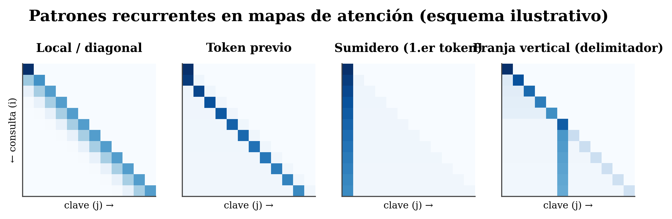
- Local / diagonal: brightness over the diagonal — the token attends to itself or to nearby neighbors.
- Previous token: a crisp diagonal shifted by one step — each token looks at the preceding one (very common and useful).
- Sink / BOS: a bright column over the first token, attended by almost everyone (see the curiosity).
- Vertical band: certain tokens —punctuation, delimiters,
[SEP]/[CLS]— receive attention from many rows. - Broad / uniform: diffuse attention, no focus.
The first-token sink is structural, not semantic (Xiao et al. 2024). Because softmax forces each row to sum to 1, when a token doesn’t need to look at anything in particular it has to dump its weight somewhere: models learn to “park” it on the first tokens. Lots of weight, little meaning. What’s more, that sink is tied to massive activations —a few enormous hidden-state values that cause it— (Sun et al. 2024; Queipo-de-Llano et al. 2025). Moral: reading the first token as “the most important one” is the most typical mistake.
14.5 Tools to see them
- BertViz (Vig 2019): interactive visualizer by layer and head.
- Attention rollout (Abnar and Zuidema 2020): since information gets mixed as it passes through layers, the raw weight of a single layer is misleading; rollout aggregates attention across layers to estimate the real flow.
- tafagent (ours): it doesn’t draw the map but instead predicts the metrics we’ll extract from it —the exponent γ, the attention horizon
d_horizon, the regime— directly from the model’s config. We’ll use it in the coming chapters.
14.6 The warning you must not forget
A map shows where the weight goes, not why the model decided something. Different attention distributions can yield the same prediction, and attention correlates poorly with true importance (Jain and Wallace 2019). A heatmap is a diagnostic, not proof of the reasoning. Don’t over-interpret it.
14.7 The bridge to measurement (what’s coming)
Beyond looking, a map can be quantified. Two questions:
- How concentrated is it? (peaky over a few tokens vs. spread out).
- How does attention decay with the distance |i−j| between tokens?
If you average many maps, a “U” shape usually appears: lots of weight at the beginning (the sink) and at the recent end, with a decaying tail in between. What we’ll measure —and, above all, what we’ll predict from the geometry of RoPE— is that tail: its decay follows a power law A(d) ∝ d^−γ.
Important (honesty). That attention decays with distance is something others observe too. What makes our Part II unique is not seeing the decay, but predicting its exponent γ from the model’s geometry (without fitting anything) and turning it into tools (compressing the KV-cache, extending the context). That’s where we’re headed in Ch. 14–15.
🧩 Analogy. Each map is a “list of glances” in a room: who looks at whom. Diagonal = everyone looks at their neighbor; previous-token = each one at the person to their left; vertical band = everyone glancing sideways at whoever presides (a delimiter); the sink = the clock on the wall, which people look at when they don’t know whom to look at (lots of glancing, no content). And there are as many lists as there are (layer, head) pairs.
14.8 Summary
- An attention map is an n×n matrix per head and per layer; there are L×H, not “one”.
- Typical patterns: local/diagonal, previous-token, sink (1st token), vertical band, broad.
- The sink is structural (softmax sums to 1 → parked weight), not importance.
- Tools: to see maps, BertViz and attention rollout (aggregates layers); to measure (γ, horizon), tafagent (Part II).
- Attention ≠ explanation: the map says where, not why.
- Quantifying the maps reveals a “U” (sink + recency + decaying tail); that tail is the law A(d)∝d^−γ we’ll measure and predict (Ch. 14–15).
Next (Chapter 14): to understand why attention loses resolution with distance, we have to look at the geometry of RoPE — aliasing and the three scales.
14.9 Exercises
- There is no “one” map. If a model has 32 layers and 32 heads, how many distinct attention maps does it produce for a sentence?
- The sink. Explain, starting from “each row sums to 1”, why a bright column appears over the first token even though it means nothing.
- Faithfulness. Why is it not valid to say “the model predicted X because this head attended to Y”?
- The U. Describe the typical shape of average attention against distance. Which part of that shape is the “sink” and which is the “tail” we’ll measure?