22 Phase structure and the polylog partition function
Where we are. We open Part III: a physical lens on attention. A warning up front, and we mean it: this is a lens, an analogy. Thermodynamics gives powerful intuition about attention, but we have to be very clear about what’s a real correspondence and what’s metaphor —and which of this is ours and which is other people’s. This chapter explains it with that honesty up front.
22.1 The idea in one sentence
The attention distribution can be read as a thermodynamic system with a “partition function”; in particular, over distance it takes the form of a polylogarithm, and γ=1 shows up as a candidate boundary between two phases.
22.2 Key concepts and their role in the transformer
Before we get into the detail, let’s define the terms of this chapter and what each one is for inside a transformer:
- Partition function Z. Definition: the “census” of a physical system —the sum over all its states weighted by
e^(−energy/temperature)—; knowing it gives you mean energy, fluctuations, etc. In the transformer: it’s the softmax normalizer of attention; here we look at it over distance between tokens, not over the context. - Polylogarithm
Li_s(z). Definition: the sum \(\sum_{k\ge1} z^k/k^s\); atz=1it’s the Riemann zetaζ(s). In the transformer: it’s the form Z takes when attention decays as a power-lawd^−γ—the generic normalizer of any power-law tail—. - Exponent γ. Definition: the rate of attention decay with distance (
A(d)∝d^−γ, Ch. 15). In the transformer: it’s the system’s control lever; it plays the role of the polylog’s exponentsand decides which phase the model is in. - Phase transition. Definition: a qualitative and abrupt change on crossing a critical value (water boiling at 100 °C). In the transformer: the framework for asking whether attention’s behavior changes suddenly on crossing γ=1.
- Hagedorn temperature. Definition: a limiting temperature (from hadron physics) above which the partition function diverges. In the transformer: the labeled analogy for the point where
Li_γstops converging —it illustrates the divergence, it doesn’t assert the literal physics—. - The γ=1 boundary (Phase A / Phase B). Definition: the value where
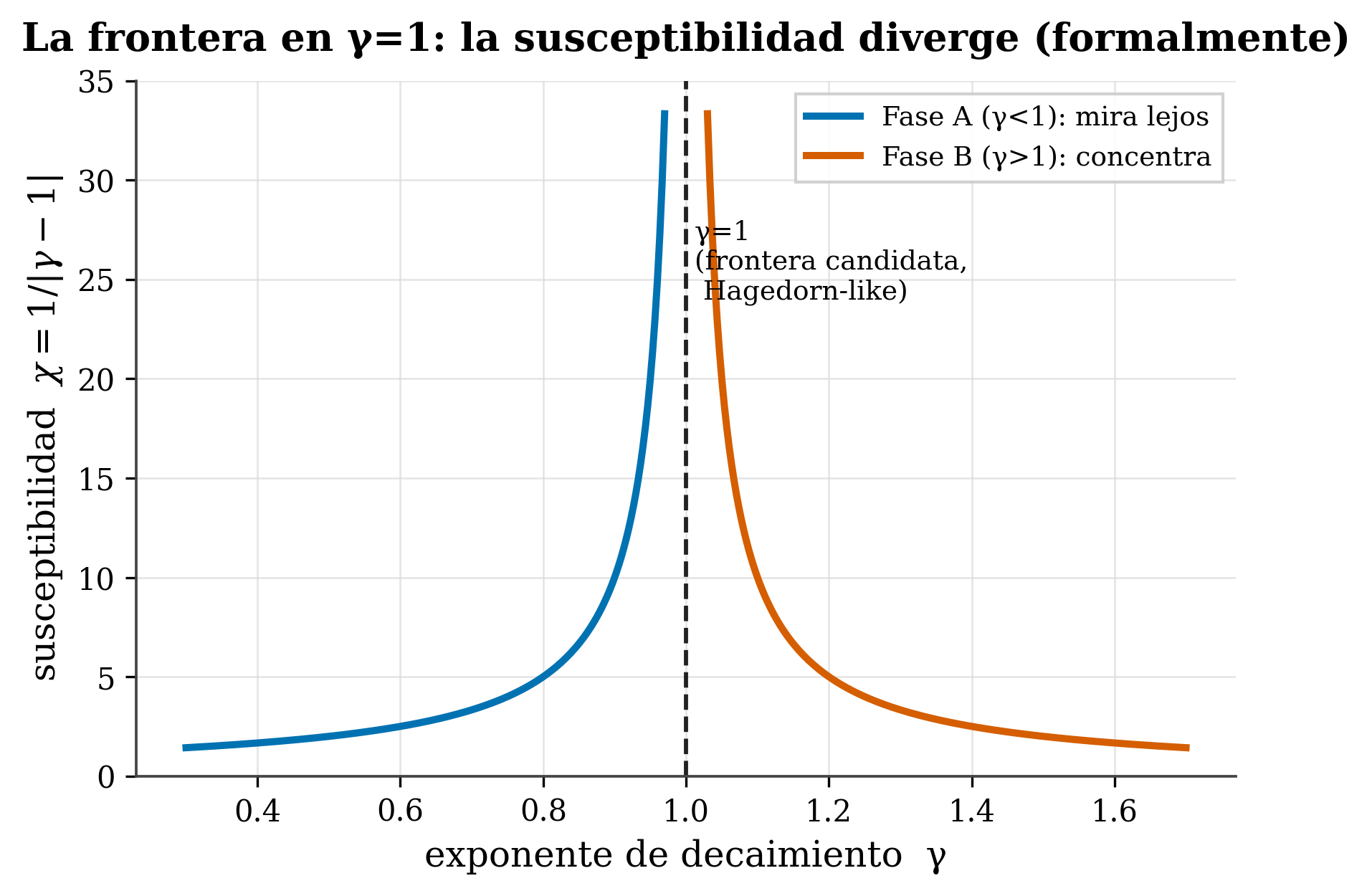
Li_1stops converging the same way, separating Phase A (γ<1, looks far) from Phase B (γ>1, concentrates). In the transformer: the candidate boundary between a model that spreads attention to the far and one that concentrates it near. - Susceptibility χ. Definition:
χ=1/|γ−1|, how much the system reacts to a tiny change of the lever. In the transformer: it blows up at γ=1, signaling that attention’s behavior changes abruptly there.
The underlying idea: read attention as a system with phases, and γ as the thermometer that tells you which side of the boundary each model is on.
22.3 The thermodynamic lens (which is NOT ours)
In physics, a partition function Z is the “census” of a system: it sums over all possible states, weighting each by e^(−energy/temperature), so that low-energy states count more. Knowing Z gives you everything (mean energy, fluctuations, etc.).
It turns out attention fits this mold: the softmax is a Boltzmann distribution (Ch. 4), with the logits as energies and an effective temperature. This we didn’t invent: it’s an active framework —the “thermodynamic isomorphism of transformers” (Kim 2026) derives the softmax by minimizing a free energy, and uses a peak in heat capacity as a precursor of grokking— on top of a decades-long tradition (Jaynes (1957); the statistical mechanics of learning of Gardner (1988), Engel and Van den Broeck (2001)). To say “we did thermodynamics of attention” would be false.
22.4 What is specifically ours: Z over distance → a polylogarithm
Our variant looks at the partition function over the distance between tokens (not over the context tokens by energy, as Kim does). If attention decays like d^−γ (Ch. 15), its normalizer takes the form of a polylogarithm:
\[ Z = \mathrm{Li}_\gamma(e^{-\lambda}), \qquad \mathrm{Li}_s(z) = \sum_{k\ge 1} \frac{z^k}{k^s} \]
What each part says:
- Z = the partition function (the “census” from before).
- Li_s(z) = the polylogarithm, which is nothing more than the sum \(\sum_{k\ge1} z^k/k^s\).
- k = the distance (the sum’s index: 1, 2, 3, …).
- s = γ = the decay exponent: each distance k weighs as
1/k^γ—exactly the power law—. - z = e^{−λ} = a factor that damps the large distances; λ acts as a “potential” (the larger λ, the less weight to the far). In the limit z→1 (λ→0),
Li_γbecomes the Riemann zetaζ(γ).
The polylogarithm Li_s is simply the generic normalizer of any power-law-tailed distribution (and at z=1 it’s the Riemann zeta ζ(s)). That “the partition function is a polylog” is automatic math if the distribution is power-law: it’s no discovery. What would add value is showing that the distance distribution really has that form and that γ is a measurable control parameter —not the name of the function—.
22.5 Phases and the Hagedorn boundary
Here’s the interesting structure. A phase transition is a qualitative and abrupt change on crossing a critical value:
🧩 Analogy. Water at 100 °C: you add heat and the temperature rises… until exactly 100 °C, where it stalls —each extra joule turns liquid into vapor instead of raising the temperature—. A lever crosses a value and the substance reorganizes all at once.
The Hagedorn temperature (from hadron physics) (Hagedorn 1965) is an extreme case: a limiting temperature above which the partition function diverges, because the number of states grows exponentially. You can’t heat past it: the extra energy creates new states instead of raising the temperature.
In our lens, γ=1 is the candidate boundary: it’s where the polylog stops converging the same way (Li_1 diverges), separating Phase A (γ<1, looks far) from Phase B (γ>1, concentrates). The susceptibility χ = 1/|γ−1| —which measures how violently the system reacts to a tiny change— blows up there (its blowing up at γ=1 signals that the behavior changes all at once):
Be careful with the name. (1) “Hagedorn” is a labeled analogy: a real Hagedorn requires exponential growth of states; we show a divergence mechanism (Li_γ as γ→1), we don’t assert the literal physics. (2) And the most delicate point: our nearest neighbor (Kim 2026) does NOT observe a divergence —it explicitly reports “no asymptotic power-law divergence… only a critical-type crossover”—. So whether γ=1 is a real transition or only a smooth crossover is an open question: at finite N, Li_1 diverges only as log N, which looks more like a crossover than a jump. We present γ=1 as a candidate boundary with evidence, not as a demonstrated transition. (3) Moreover, our own calculation of the heat capacity at γ=1 had an erratum (a factor of 12 vs 4) that we corrected and verified in Lean —we tell that story in Ch. 22—.
22.6 Why this lens isn’t just decoration
Despite the caveats, the physics connects to the practical: γ=1 is exactly the KV-cache compressibility boundary (Ch. 20) —the point where the polylog stops converging is the same one where a finite window stops capturing the mass—. The thermodynamic lens and the engineering tool point at the same threshold. That’s what makes the analogy valuable: not because it sounds elegant, but because it predicts where things change.
tafagent classifies your model into Phase A or B relative to the γ=1 line and reports the susceptibility χ. You’ll see that the atlas models (Ch. 16) cluster just below γ=1 —close to that boundary—.
22.7 Summary
- The thermodynamic lens reads the softmax as Boltzmann and defines a partition function Z. It’s not ours (Kim (2026) + the Jaynes/Gardner tradition).
- Ours: Z over distance → polylog form
Z=Li_γ(e^−λ); γ=1 as a candidate boundary (Phase A/B), with χ=1/|γ−1| diverging there. - Honest: the polylog is the automatic normalizer of a power-law; “Hagedorn” is an analogy; and whether γ=1 is a transition or only a crossover is open (the neighbor doesn’t see a divergence); + our own erratum in C_V(γ=1), corrected in Lean.
- Value: γ=1 coincides with the KV compressibility boundary (Ch. 20) — the physics points at the same threshold as the practice.
Next (Chapter 22): the full thermodynamic “dictionary” —temperature, heat capacity, Fisher information— and the identity that is verified in Lean: Fisher = C_V.
22.8 Exercises
- Partition function. In one sentence: what does Z “census,” and why does knowing it give you everything?
- The polylog. Why do we say that “Z is a polylog” isn’t, by itself, a discovery?
- Transition vs crossover. What’s the difference between a phase transition (water at 100 °C) and a smooth crossover (butter softening)? Which one does the neighbor Kim see?
- Honesty. Why do we call γ=1 a “candidate boundary” and not a “demonstrated phase transition”?