17 The γ atlas: decay measured across 42 models
Where we are. In Ch. 15 we learned to measure (and to predict) a model’s decay exponent γ. The natural question: if we can measure it in one, let’s measure it in many. That’s the γ atlas —γ measured across 42 models from four architecture families (Marín 2026)— and it’s something no other manual has: a common map where to place any transformer by how it attends across distance. This chapter explains the map calmly, what it tells us, and —with the same honesty as always— what we cannot conclude from it.
17.1 The idea in one sentence
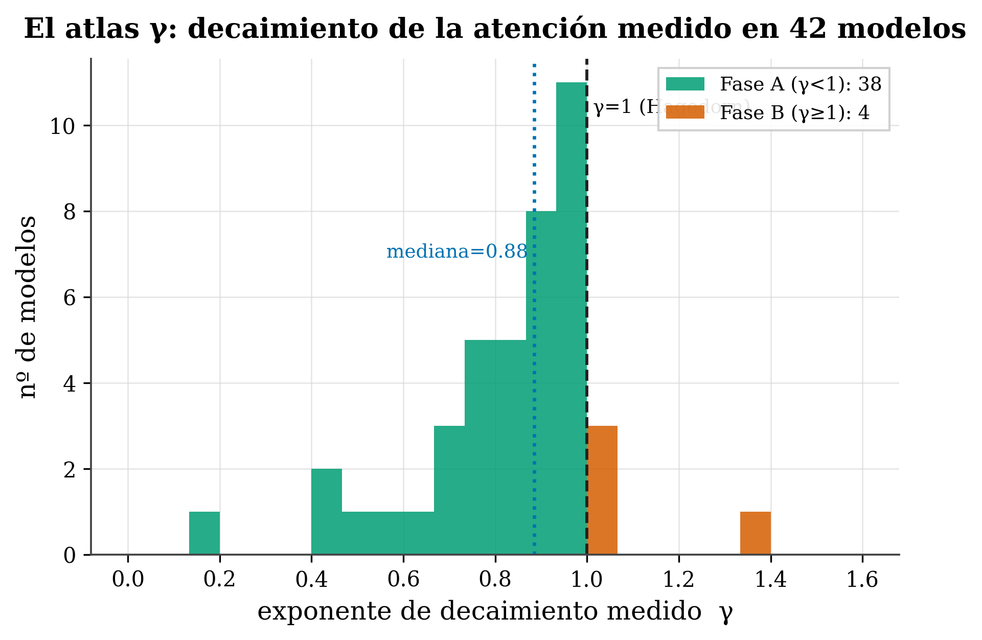
With γ measured across 42 different models, a map emerges: most trained transformers look far (γ<1), with a median near —but below— the boundary γ=1.
17.2 Key concepts and their role in the transformer
Before getting into detail, we define this chapter’s terms and what each one is for inside a transformer:
- γ atlas. Definition: the decay exponent γ measured across 42 models from four architecture families. In the transformer: it turns γ from a property of one model into a common map where to place and compare them all.
- γ as a comparable coordinate. Definition: a single number that places very different models (dense, GQA, MoE, SSM) on the same axis. In the transformer: it lets you compare how they attend across distance regardless of architecture.
- Phase A (γ<1) and Phase B (γ>1). Definition: a heavy tail that looks far (Phase A) versus attention that concentrates close (Phase B). In the transformer: it indicates whether the model exploits broad context or not — key for KV-cache compression (Ch. 20).
- Hagedorn boundary (γ=1). Definition: the line that separates the two phases. In the transformer: models cluster just below it (median ≈0.885), a pattern that doesn’t look accidental and is revisited in Ch. 21.
- Cross-architecture. Definition: that γ is the same kind of measurement for dense, GQA, MoE and SSM models. In the transformer: it’s what makes the atlas unique — it puts a Mamba and a GPT on the same axis.
- R² of the fit. Definition: how well
A(d)∝d^−γdescribes the real attention of each model (high = good fit). In the transformer: it signals when γ is a reliable summary and when it’s coarser (R²~0.85). - Raw γ vs. within-model control. Definition: comparing γ as-is across models mixes factors (θ, data, architecture); the clean experiment varies θ within the same model. In the transformer: the atlas describes the landscape but doesn’t isolate causes on its own.
In short: the atlas is a reproducible snapshot of the γ landscape, not an eternal law nor a causal proof.
17.3 What an atlas is for
Up to now γ was a property of one model. But measuring it across many turns it into a comparable coordinate: a single number that places models as different as a dense GPT, one with GQA, a Mixture-of-Experts or even a state-space model (Mamba) on the same axis. It’s like going from measuring the temperature of a city to having the weather map of a whole country: what’s interesting isn’t a point, it’s the pattern they all draw together.
17.4 The map
figures/make_fig16_atlas.py over data/gamma_atlas.csv.
17.5 What the map tells us (calmly)
Three readings, and what each one means:
1. Almost all look far (38 of 42 in Phase A, γ<1). This is telling. Recall (Ch. 15) that γ<1 means heavy tail: attention falls off slowly with distance, so the model also spreads weight to far-off tokens. That the vast majority of trained models end up there suggests that exploiting broad context is the norm, not the exception —transformers, left to their own devices, tend toward the long gaze, not tunnel vision—.
2. The median (γ≈0.885) is near the boundary, but below it. Models don’t distribute at random: they cluster just below γ=1. It’s as if training pushed them toward the edge of the “look far” regime without quite crossing it. That closeness to the boundary (the “Hagedorn transition” of Ch. 21) is no coincidence and we’ll revisit it.
3. There’s real diversity (range γ ≈ 0.15 → 1.34). Not all are alike: there are very heavy-tailed models (γ≈0.15, extremely long gaze) and a few in Phase B (γ>1) that concentrate close. That range is what connects with practical decisions: how much context a model truly exploits, how much its KV-cache can be compressed (Ch. 20).
17.6 The unique piece: it’s cross-architecture
What makes the atlas special is not just the number of models, but that γ is the same kind of measurement for very different architectures —dense, GQA, MoE and SSM—. Few diagnostics let you put a Mamba and a GPT on the same axis. γ does.
Three cautions, so as not to over-interpret: 1. Comparing raw γ across very different models mixes factors. Two 7-8B models can differ in γ because of their θ, their data and their architecture all at once (the decomposition of Ch. 15). The clean experiment —which does control everything— is to vary θ within the same model (we’ll see it with sinks, Ch. 17). The atlas describes; it doesn’t isolate causes on its own. 2. The quality of the fit varies. The law d^−γ fits very well in general (R²>0.95 in many), but in some models the R² is lower (~0.85): there γ is a coarser summary. We indicate it model by model (the R2 column of the dataset). 3. It’s a snapshot, not a universal law. 42 models at a given moment; an atlas gets expanded and corrected. The data are published so anyone can reproduce it and discuss it.
17.7 Where the data come from
The atlas is measured with a reproducible procedure (fitting A(d)∝d^−γ over the real attention of each model) and is published as an open dataset —so you don’t have to take anything on faith: it can be downloaded, reproduced, criticized—. (The detail of how to measure your own γ is in the reference cookbook, R4.)
tafagent has a Phase diagram mode that places a panel of models on the γ axis (Phase A vs Phase B), and when you profile your model it tells you where in the atlas it falls. It’s the atlas made interactive: add yours and compare it.
17.8 Summary
- The γ atlas measures the decay exponent across 42 models from 4 families —a cross-architecture coordinate nobody else has—.
- Reading: 38 of 42 in Phase A (γ<1, look far) → exploiting broad context is the norm; median ≈0.885 (they cluster just below the γ=1 boundary); range 0.15–1.34 (real diversity).
- Unique: γ puts dense, GQA, MoE and SSM on the same axis.
- Honest: raw cross-model γ mixes factors (the clean control is within-model, Ch. 17); the R² varies; it’s a reproducible snapshot, not an eternal law.
Next (Chapter 17): one of those “raw readings” is misleading —concentration (sinks)—. We’ll see it’s independent of γ, with the clean experiment that controls everything: the θ-rescale within the same model.
17.9 Exercises
- Reading the map. If 38 of 42 models have γ<1, what do trained transformers tend to do: look far or concentrate close? Why?
- The median. What’s striking about models clustering just below γ=1 instead of spreading across the whole range?
- Honesty. Why is comparing the γ of two different models not enough to say “this one looks farther because of its architecture”? What experiment would isolate it?
- Fit. If a model has R²=0.85 in its γ fit, how much confidence would you place in its γ versus another with R²=0.98?
The complete γ atlas and the per-model data on which this chapter is based are open: Predicting How Transformers Attend (Zenodo).